
Estimating Street Safeness after an Earthquake with Computer Vision And Route Planning
April 28, 2020

We answered how to estimate the safest route after an earthquake with computer vision and route management.
The problem
The last devastating earthquake in Turkey occurred in 1999 (>7 on the Richter scale) around 150–200 kilometers from Istanbul. Scientists believe that this time the earthquake will burst directly in the city and the magnitude is predicted to be similar.
The main motivation behind this AI project hosted by Impacthub Istanbul is to optimize the Aftermath Management of Earthquake with AI and route planning.
Children need their parents!
After kicking off the project and brainstorming with the hosts, collaborators, and the Omdena team about how to better prepare the city of Istanbul for an upcoming disaster, we spotted a problem quite simple but at the same time really important for families: get reunited ASAP in earthquake aftermath!
Our target was set to provide safe and fast route planning for families, considering not only time factors but also broken bridges, landing debris, and other obstacles usually found in these scenarios.
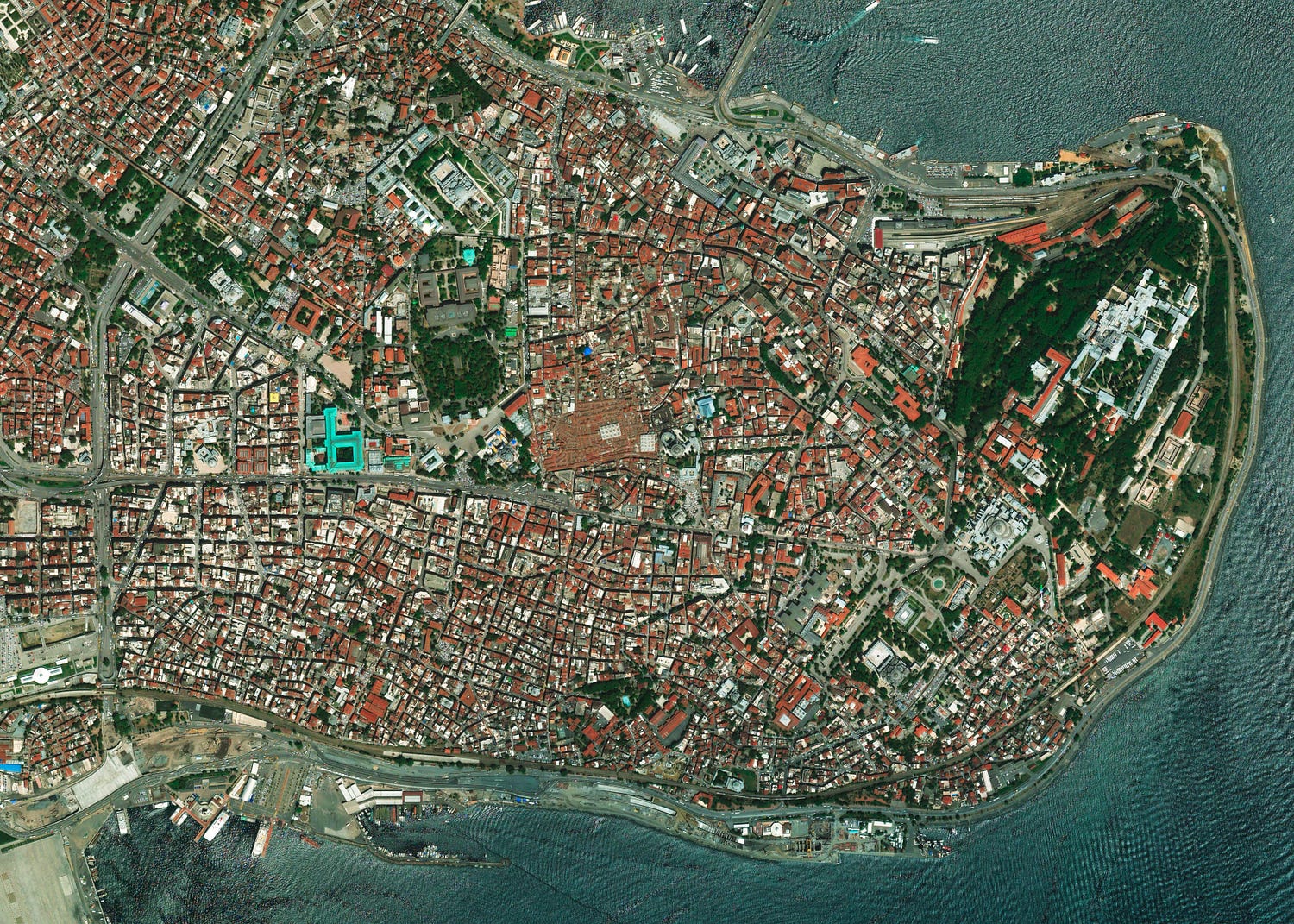
Fatih, one of the most popular and crowded districts in Istanbul. Source: Mapbox API
We resorted to working on two tasks: creating a risk heatmap that would depict how dangerous is a particular area on the map, and a path-finding algorithm providing the safest and shortest path from A to B. The latter algorithm would rely on the previous heatmap to estimate safeness.
Challenge started! Deep Learning for Earthquake management by the use of Computer Vision and Route Management.

Source: Unsplash @loic
By this time, we optimistically trusted in open data to successfully address our problem. However, we realized soon that data describing buildings quality, soil composition, as well as pre and post-disaster imagery, were complex to model, integrate, when possible to find.
Bridges over streets, buildings height, 1000 types of soil, and eventually, interaction among all of them… Too many factors to control! So we just focused on delivering something more approximated.
Computer Vision and Deep Learning is the answer for Earthquake management
The question was: how to accurately estimate street safeness during any Earthquake in Istanbul without such a myriad of data? What if we could roughly estimate path safeness by embracing distance-to-buildings as a safety proxy. The farther the buildings the safer the pathway.
For that crazy idea, firstly we needed buildings footprints laid on the map. Some people suggested borrowing buildings footprints from Open Street Map, one of the most popular open-source map providers. However, we noticed soon Open Street Map, though quite complete, has some blank areas in terms of buildings metadata which were relevant for our task. Footprints were also inaccurately laid out on the map sometimes.
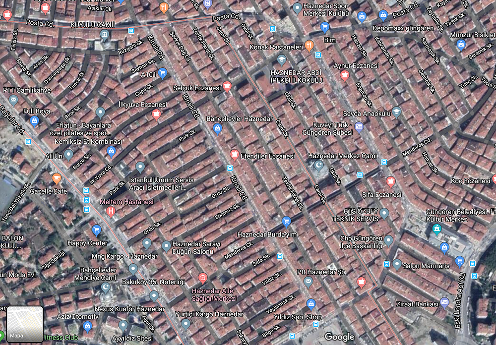
Haznedar area (Istanbul). Source: Satellite image from Google Maps.
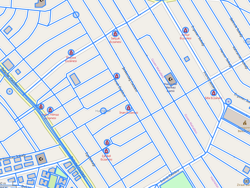
Haznedar area too, but few footprints are shown. Blue boxes depict building footprints. Source: OpenStreetMap.
A big problem regarding the occurrence of any Earthquake and their effects on the population, and we have Computer Vision here to the rescue! Using Deep Learning, we could rely on satellite imagery to detect and then, estimated closeness from pathways to them.
The next stone on the road was to obtain high-resolution imagery of Istanbul. With enough resolution to allow an ML model locates building footprints in the map as a standard-visually-agile human does. Likewise, we would also need some annotated footprints on these images so that our model can gracefully train.
First step: Building a detection model with PyTorch and fast.ai
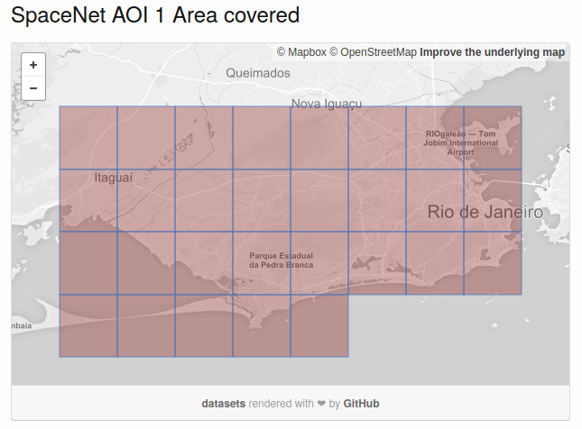
SpaceNet dataset covering the area for Rio de Janeiro. Source: https://spacenetchallenge.github.io/
Instead of labeling hundreds of square meters manually, we trusted on SpaceNet (and in particular, images for Rio de Janeiro) as our annotated data provider. This dataset contains high-resolution satellite images and building footprints, nicely pre-processed and organized which were used in a recent competition.
The modeling phase was really smooth thanks to fast.ai software.
We used a Dynamic Unit model with an ImageNet pre-trained resnet34 encoder as a starting point for our model. This state-of-the-art architecture uses by default many advanced deep learning techniques, such as a one-cycle learning schedule or AdamW optimizer.
All these fancy advances in just a few lines of code.
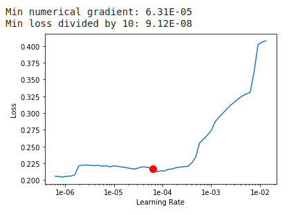
fastai fancy plot advising you about learning rates.
We set up a balanced combination of Focal Loss and Dice Loss, and accuracy and dice metrics as performance evaluators. After several frozen and unfrozen steps in our model, we came up with good-enough predictions for the next step.
For more information about working with geospatial data and tools with fast.ai, please refer to [1].
Where is my high-res imagery? Collecting Istanbul imagery for prediction.
Finding high-resolution imagery was the key to our model and at the same time a humongous stone hindering our path to victory.
For the training stage, it was easy to elude the manual annotation and data collection process thanks to SpaceNet, yet during prediction, obtaining high-res imagery for Istanbul was the only way.

Mapbox sexy logo
Thankfully, we stumble upon Mapbox and its easy-peasy almost-free download API which provides high-res slippy map tiles all over the world, and with different zoom levels. Slippy map tiles are 256 × 256 pixel files, described by x, y, z coordinates, where x and y represent 2D coordinates in the Mercator projection, and z the zoom level applied on earth globe. We chose a zoom level equal to 18 where each pixel links to real 0.596 meters.
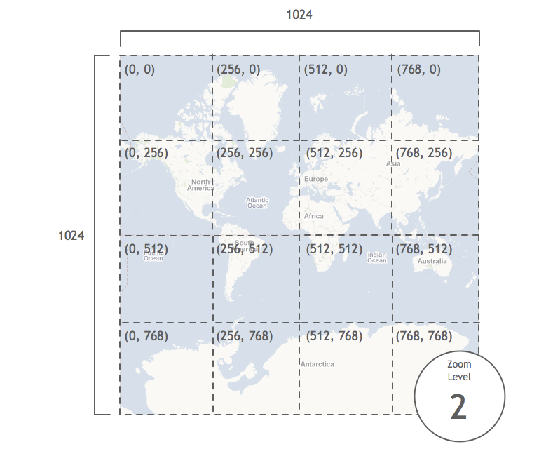
Slippy map tiles on the Mercator projection (zoom level 2). Source: http://troybrant.net/blog/2010/01/mkmapview-and-zoom-levels-a-visual-guide/
As they mentioned on their webpage, they have a generous free tier that allows you to download up to 750,000 raster tiles a month for free. Enough for us as we wanted to grab tiles for a couple of districts.
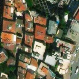
Slippy raster tile at zoom level 18 (Fatih, Istanbul).
Time to predict: Create a mosaic-like your favorite painter
Once all required tiles were stealing space from my Google Drive, it was time to switch on our deep learning model and generate prediction footprints for each tile.
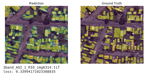
Model’s prediction for some tile in Rio: sometimes predictions looked better than actual footprints.
Then, we geo-referenced the tiles by translating from the Mercator coordinates to the latitude-longitude tuple (that used by mighty explorers). Geo-referencing tiles was a required step to create our prediction piece of art with GDAL software.
Python snippet to translate from Mercator coordinates to latitude and longitude.
Concretely, gdal_merge.py thecommand allows us to glue tiles by using embedded geo-coordinates in TIFF images. After some math, and computing time… voilà! Our high-res prediction map for the district is ready.
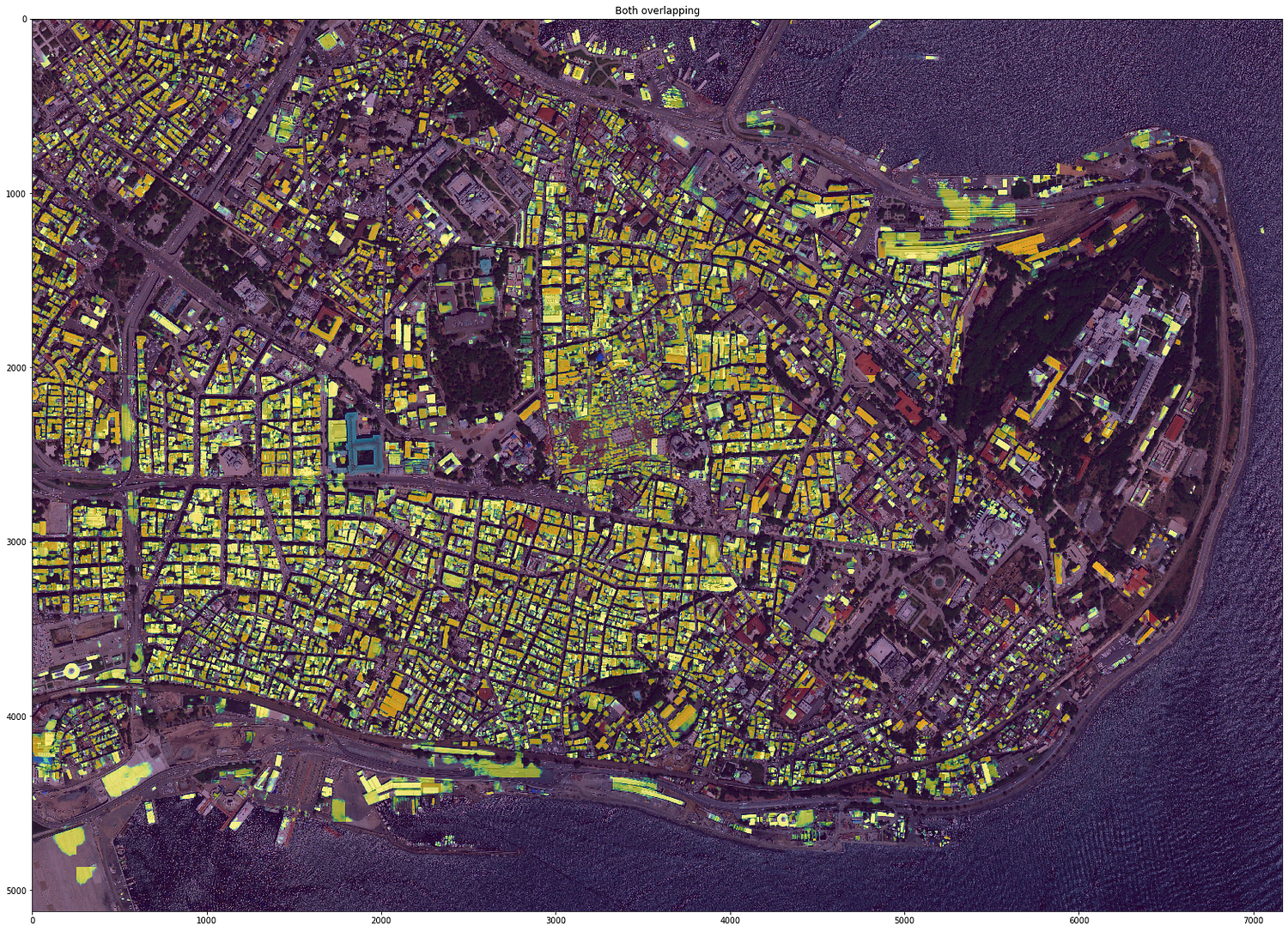
Raw predictions overlaid on Fatih. From a lower degree of building presence confidence (blue) to higher (yellow).
Inverse distance heatmap
Ok, I see my house but should I go through this street?
Building detection was not enough for our task. We should determine distance from a given position in the map to the closest building around so that a person in this place could know how safe is going to be to cross this street. The larger the distance the safer, remember?
The path-finding team would overlay the heatmap below on his graph-based schema and by intersecting graph edges (streets) with heatmap pixels (user positions), they could calculate the average distance for each pixel on the edge and thus obtaining a safeness estimation for each street. This would be our input when finding the best A-B path.
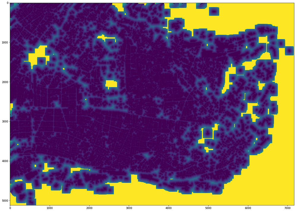
Distance-to-buildings heatmap in meters. Each pixel represents the distance from each point to the closest building predicted by our model. Blue means danger, yellow-green safeness.
But how to produce this picture from the raw prediction map? Clue: computing distance pixel-building for each tile independently is sub-optimal (narrow view), whereas the same computation on the entire mosaic will render as extremely expensive (3.5M of pixels multiplied thousands of buildings).
Working directly on the mosaic with a sliding window was the answer. Thus, for each pixel (x,y), a square matrix composed by (x-pad, y-pad, x+pad, y+pad) pixels from the original plot is created. Pad indicates the window side length in the number of pixels.
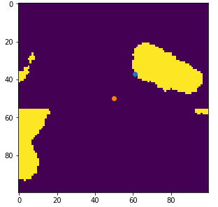
Pixel-wise distance computation. Orange is the point, blue is the closest building around. Side length = 100 pixels.
If a pixel belongs to some building, it returns zero. If not, return the minimum euclidean distance from the center point to the building’s pixels. This process along with NumPy optimizations was the key to mitigate the quadratic complexity beneath this computation.
Repeat the process for each pixel and the safeness map comes up.
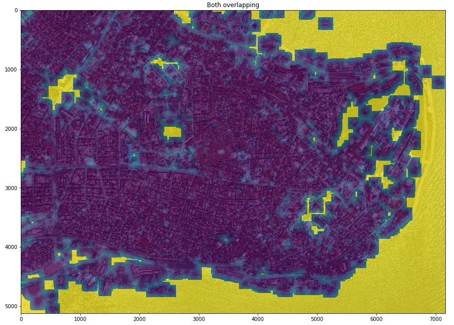
Distance heatmap overlaid on the satellite image. Blue means danger, yellow-green safeness.
- Harnessing AI and Open Source Satellite Imagery to Address Global Problems
- Object Detection for Preventing Road Crashes and Saving Lives
Want to work with us?
If you want to discuss a project or workshop, schedule a demo call with us by visiting: https://form.jotform.com/230053261341340
Related Articles


