the Creative Commons Attribution 4.0 License.
the Creative Commons Attribution 4.0 License.
 | 03 Aug 2021
Thermal legacy of a large paleolake in Taylor Valley, East Antarctica, as evidenced by an airborne electromagnetic survey
Krista F. Myers
Peter T. Doran
Slawek M. Tulaczyk
Neil T. Foley
Thue S. Bording
Esben Auken
Hilary A. Dugan
Jill A. Mikucki
Nikolaj Foged
Denys Grombacher
Ross A. Virginia
Previous studies of the lakes of the McMurdo Dry Valleys have attempted to constrain lake level history, and results suggest the lakes have undergone hundreds of meters of lake level change within the last 20 000 years. Past studies have utilized the interpretation of geologic deposits, lake chemistry, and ice sheet history to deduce lake level history; however a substantial amount of disagreement remains between the findings, indicating a need for further investigation using new techniques. This study utilizes a regional airborne resistivity survey to provide novel insight into the paleohydrology of the region. Mean resistivity maps revealed an extensive brine beneath the Lake Fryxell basin, which is interpreted as a legacy groundwater signal from higher lake levels in the past. Resistivity data suggest that active permafrost formation has been ongoing since the onset of lake drainage and that as recently as 1500–4000 years BP, lake levels were over 60 m higher than present. This coincides with a warmer-than-modern paleoclimate throughout the Holocene inferred by the nearby Taylor Dome ice core record. Our results indicate Mid to Late Holocene lake level high stands, which runs counter to previous research finding a colder and drier era with little hydrologic activity throughout the last 5000 years.


Lakes provide a refuge to life in some of the more extreme environments on Earth, especially in places with strong seasonality such as polar regions. Lakes are a relatively stable source of liquid water which can determine the ecological viability of a system (Gooseff et al., 2017). The evolution of lake basins is important to survival of local ecosystems, and interpreting the history of lake levels and water availability can provide important insights into long-term ecosystem dynamics. Despite extremely low temperatures and minimal precipitation, the McMurdo Dry Valleys (MDVs; Fig. 1) are the site of a series of closed-basin lakes fed by alpine glacial melt and snowmelt via ephemeral streams as well as by direct subsurface recharge (Toner et al., 2017; Lawrence et al., 2020). Annual lake levels in the MDVs have been recorded since the 1970s, which provides a window into the dynamic climatic and geologic drivers of the MDV hydrologic system (Fountain et al., 2016). Lake levels have overall risen since the beginning of observational records starting in 1903, during Robert Scott's first expedition (Scott, 1905); however periods of lake level stagnation as well as lake level drop have also been recorded (Fountain et al., 2016). The fluctuation in the MDV lakes alters the biological and chemical exchange between surface waters, soils, and groundwater, making it critical for understanding MDV connectivity and ecosystem evolution (Doran et al., 2002a; Gooseff et al., 2017; Foley et al., 2019).
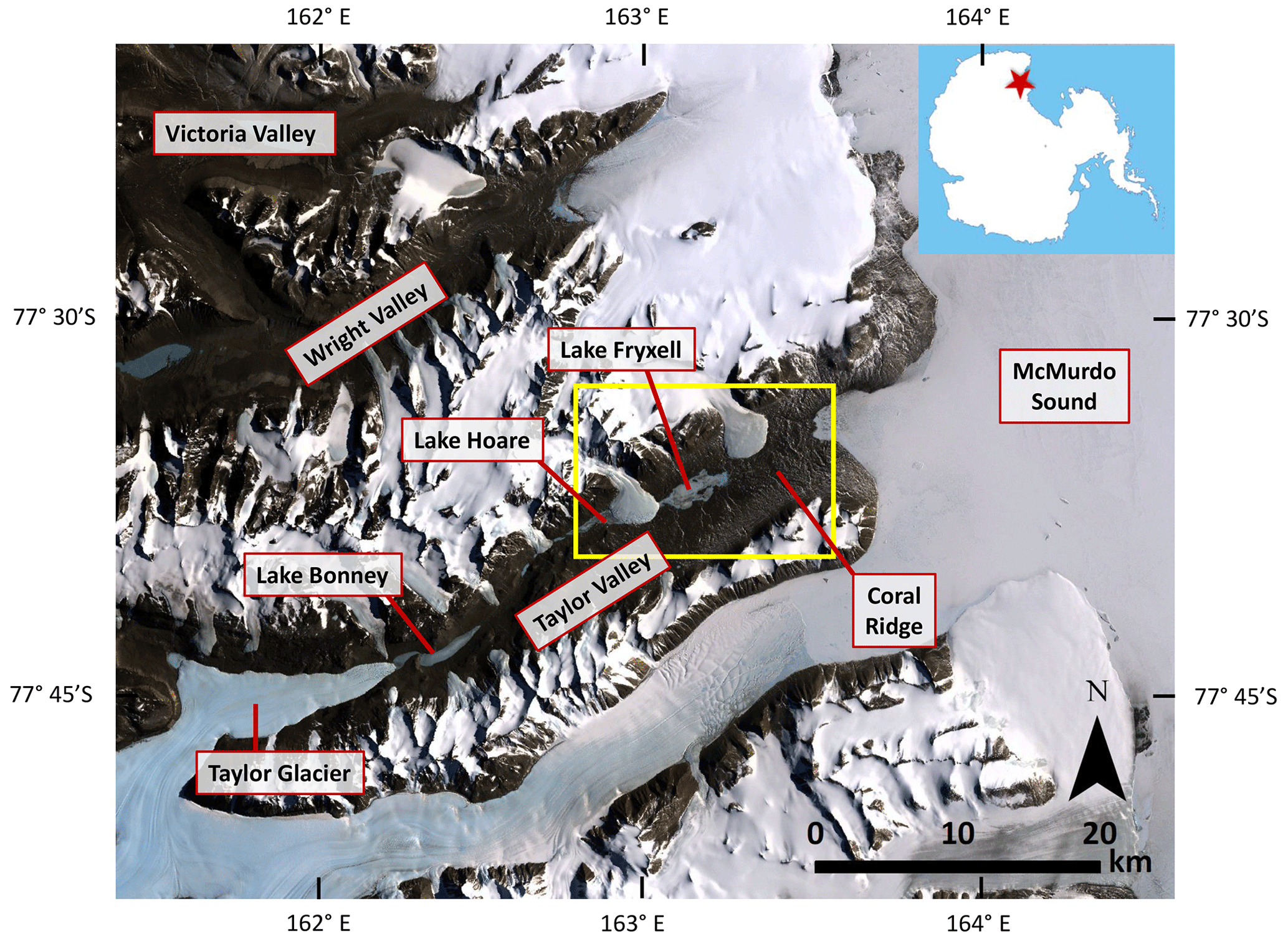
Figure 1Overview map of the McMurdo Dry valleys. Lake Fryxell is located in the eastern portion of Taylor Valley, and the study area is outlined in yellow. Satellite imagery from Landsat Imagery Mosaic Antarctica (LIMA) published 2009.
The drivers of MDV lake level change represent a complex combination of climate, ice sheet extent, and basin hypsometry. During the Last Glacial Maximum (LGM), roughly 28.5–12.8 ka, Antarctica underwent a period of ice sheet thickening and advance (Hall et al., 2015). Stable isotope records from Taylor Dome (located roughly 100 km west of the MDVs) indicate mean annual air temperatures ca. 4–9 ∘C lower than modern during the LGM (Steig et al., 2000). Following the LGM (12 000–2000 years BP) regional temperatures were up to 5 ∘C warmer than modern conditions (Fig. 2) (Steig et al., 2000; Monnin et al., 2004). During the LGM, ice from the East and West Antarctic ice sheets was grounded within the Ross Sea, extending to the edge of the continental shelf, roughly 500 km farther than the modern-day grounding line (Anderson et al., 2014). Grounded ice from the Ross Ice Shelf flowed inland, spilled into the ice-free MDVs, and formed an ice dam that reached approximately 350 m above sea level (m a.s.l.) (Denton and Marchant, 2000). The grounded Ross Ice Shelf in the mouth of Taylor Valley (TV) would have allowed for lake levels to reach elevations that would otherwise not be possible (∼300–350 m a.s.l.), forming a massive glacially dammed lake known as Glacial Lake Washburn (GLW), which would have filled all of TV (Fig. 3a). According to Hall and Denton (2000), the Ross Ice Shelf remained grounded at a maximum equilibrium extent along the eastern side of the Transantarctic Mountains until roughly 13 067 years BP (12 700 14C years BP, calibrated using Stuiver et al., 2018).
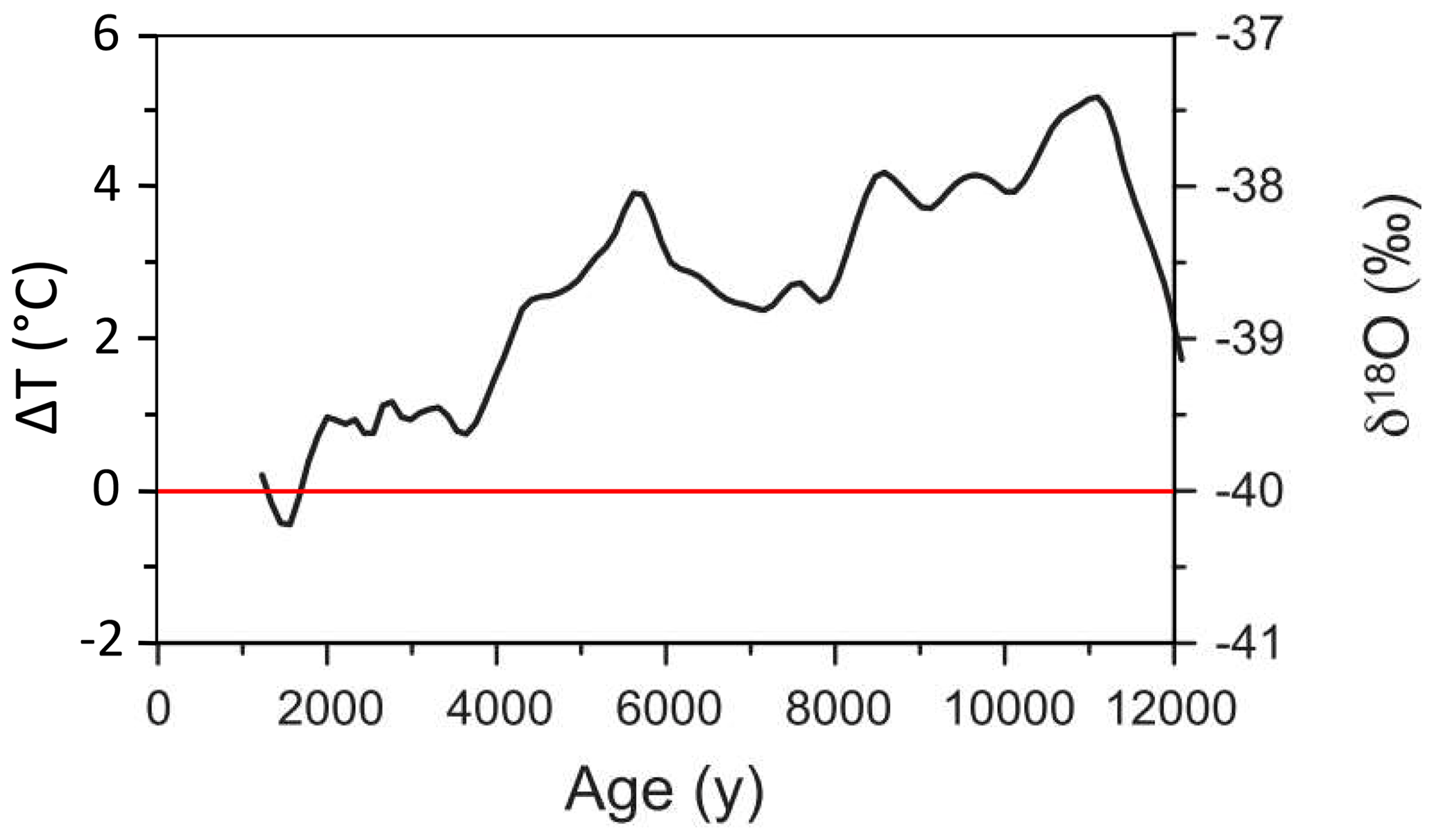
Figure 2Stable isotope (δ18O) record from Taylor Dome ice core and paleotemperature reconstruction. A reference line for 0 ΔT (∘C) is shown in red, representing deviation from modern temperatures. Modified from Monnin et al. (2004).
The removal of the ice dam in the mouth of TV would have resulted in drainage of GLW, and subsequent lake levels would be limited by the 78–81 m a.s.l. topographic constraint (outflow sill) at Coral Ridge (Fig. 3b). However, the exact date that the ice dam was removed is still not completely resolved in the literature. Some studies suggest the grounded ice sheet was completely gone from the mouth of TV sometime between 7800 to 6000 years BP (Cunningham et al., 1999; Hall et al., 2006, 2013; Anderson et al., 2016). However, grounded ice could have persisted in the mouth of TV after the Ross Ice Shelf retreated. Levy et al. (2017) used luminescence dating to suggest that large paleolakes in neighboring Garwood Valley persisted well after the Ross Ice Shelf retreated. The paleolake Howard (Garwood Valley) was at its maximum elevation until 4.26±0.72 ka because of stranded ice in the mouth of Garwood Valley that was a relic of the Ross Ice Shelf. Levy et al. (2017) makes the case that relic ice could have persisted in the mouths of various valleys well after the Ross Ice Shelf retreated in McMurdo Sound, so ice shelf retreat may not correlate exactly with the timing of GLW drainage. Other studies (Horsman, 2007; Arcone et al., 2008; Toner et al., 2013) suggested that GLW was much smaller and only occupied western TV in the Lake Bonney basin.
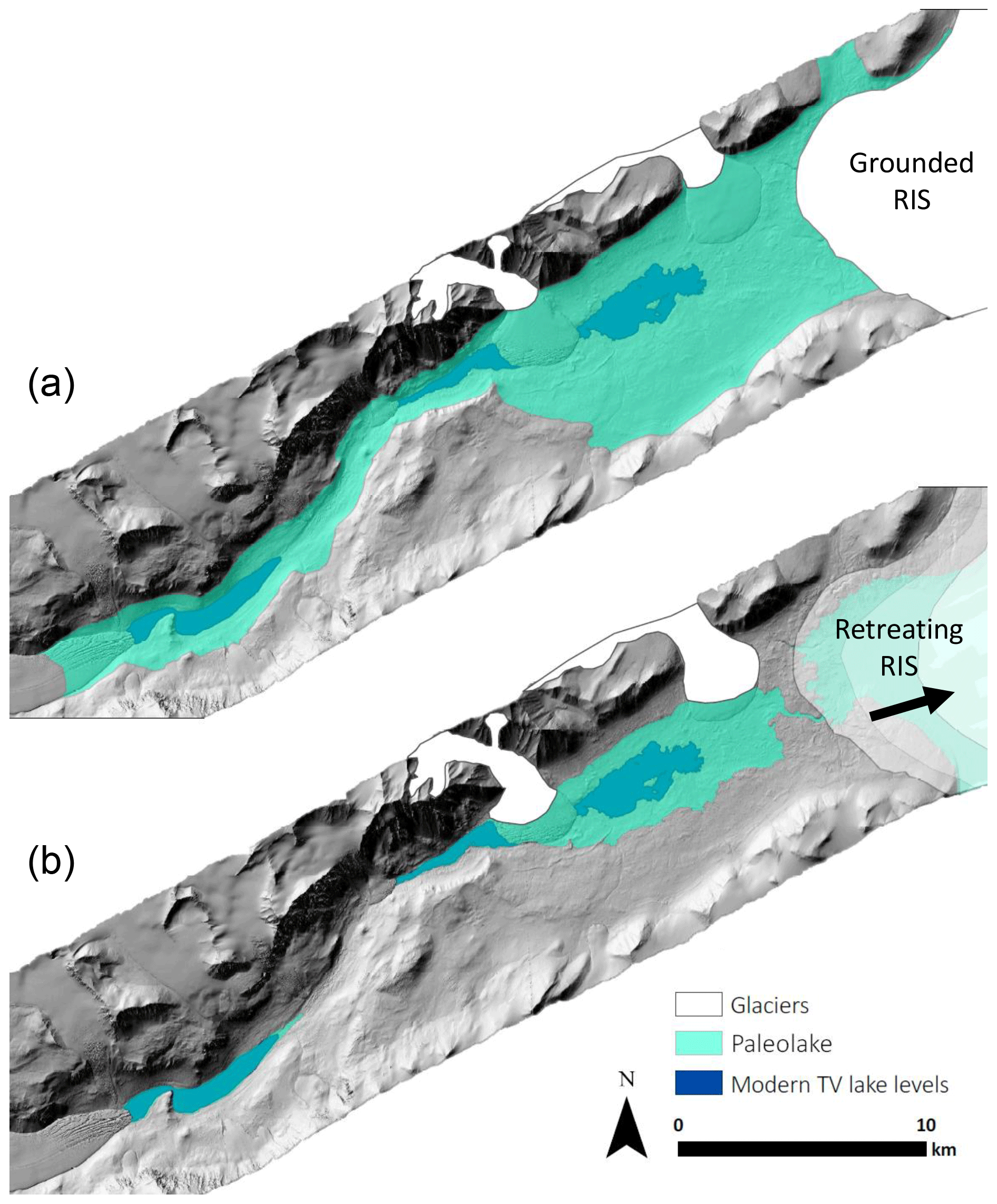
Figure 3(a) Glacial Lake Washburn extending up Taylor Valley (300 m a.s.l.). Extent of grounded Ross Ice Sheet is estimated from maps of Ross Sea drift moraine locations (Hall and Denton, 2000); (b) Holocene extent of paleolake, limited by 81 m a.s.l. sill between Lake Fryxell and the McMurdo Sound. Modern-day lake levels shown in dark blue. Extent of alpine glaciers (Canada and Commonwealth glaciers in white) is estimated. The DEM (1 m resolution) is from 2014–15 lidar survey, accessed via OpenTopography (Fountain et al., 2017).
Much of the past lake level chronology in TV has been established by dating paleodeltas, which form where streams enter the lake and deposit sediment. Previous studies have utilized radiocarbon dating of algal mats within these deltas (Hall and Denton, 2000) and optically stimulated luminescence (OSL) dating of quartz grains (Berger et al., 2013) to constrain the age of the paleodeltas. Hall and Denton (2000) postulate that a large lake occupied the full TV, reaching an elevation of up to 350 m a.s.l., between a period of 8340 and 23 800 years BP, suggesting lake levels dropped below modern levels by 8 ka (Fig. 4). Berger et al. (2013) determined that delta deposits are systematically younger than the 14C dates at comparable elevations by ∼5000 years (Fig. 4), suggesting a lake level drop below sill level between 5 and 8 ka.
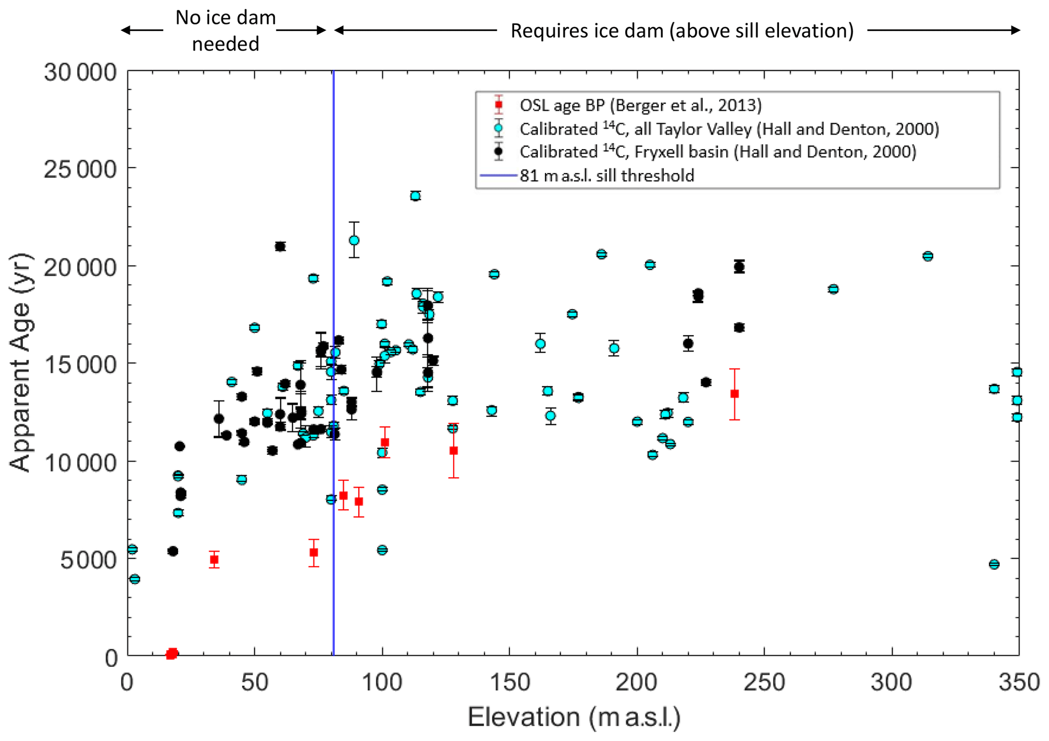
Figure 4Age of delta deposits from 14C dating of preserved algal mats (Hall and Denton, 2000) shown as circles with associated error bars (age). Samples from all of Taylor Valley and just Fryxell basin shown as cyan and black circles, respectively. Age estimates using optically stimulated luminescence (OSL) dating shown as red squares with associated error bars (age) (Berger et al., 2013). The vertical blue line represents approximate elevation of sill at Coral Ridge (81 m a.s.l.), defining the elevation at which any lake level above would require an ice dam. The calibrated 14C ages from Hall and Denton (2000) were corrected using the CALIB program (Stuiver et al., 2018).
The disagreement of spatial distribution and timing of paleolake levels in TV highlights the need to further constrain lake level history. This study provides a third method for estimating lake level history during the previously unconstrained Mid to Late Holocene (5 ka to present) using a novel application of electrical resistivity data to identify the subsurface thermal legacy of paleolake levels in TV.
The MDVs are located within the Transantarctic Mountains and make up the largest ice-free region in Antarctica (Levy, 2013). Mean annual valley bottom temperatures in TV range from −14.7 to −23.0 ∘C (Obryk et al., 2020), and the region receives between 3–50 mm water equivalent of precipitation per year (Fountain et al., 2010). Lakes in the MDVs have 3–5 m thick perennial ice covers and vary in volume, chemistry, and biological activity (Lyons et al., 2000). During the austral summer, a short melt window occurs between December and February, which accounts for most of the stream input to the lakes (Chinn, 1987). Open-water moats form around the perimeter of the lakes during the summer, and water loss occurs due to sublimation of lake ice and evaporation of open water (Dugan et al., 2013; Obryk et al., 2017).
Lake Fryxell, located in TV, is one of the largest lakes in the MDVs, at roughly 5.5 km long, 1.75 km wide, and 22 m deep (Fig. 1). Lake level measurements show that from 1972 to 2020, Lake Fryxell has undergone ∼2.61 m of total lake level rise as measured by manual lake level surveys at an average rate of ∼5.4 cm yr−1 (Fig. 5) (Doran and Gooseff, 2020). The lake level record is characterized by high interannual variability in both lake level change (magnitude) and direction (rise versus fall) (Fountain et al., 2016).
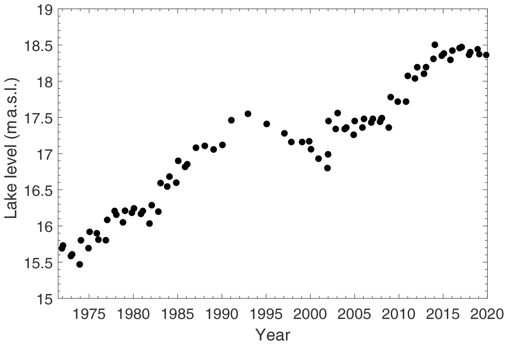
Figure 5Lake level elevation in meters above sea level (m a.s.l.) of Lake Fryxell from 1972 to 2020. Lake levels are determined by manual survey. Data can be accessed at https://mcm.lternet.edu (last access: 16 July 2020; Doran and Gooseff, 2020).
2.1 Resistivity surveys
SkyTEM, a time domain airborne electromagnetic sensor system, was flown over TV in 2011 (see Fig. 6 for SkyTEM data collection flight lines). The measurement involves pulsing a strong current in a transmitter coil suspended beneath a helicopter. When these currents are turned off rapidly, a primary magnetic field propagates throughout the subsurface, which induces eddy currents in the subsurface at depth. The decay of these eddy currents in turn generates a secondary magnetic field, the strength and time dependence of which are measured inductively by a receiver coil that is also suspended beneath the helicopter (Foley et al., 2016). The resulting data, which consist of time derivatives of the secondary magnetic field, are used to estimate the resistivity in the subsurface (Ward and Hohmann, 1988). Data collection occurs while the helicopter flies at speeds up to approximately 100 km h−1. The 2011 airborne electromagnetic survey collected 560 km of resistivity data in eastern TV. Flight lines were approximately 500 m apart, and nodes (individual sounding points) were collected every ∼25 m along each flight line (Fig. 6). For more details and in-depth discussion behind SkyTEM methodology and data collection, see Sørensen and Auken (2004), Mikucki et al. (2015), and Foley et al. (2016).
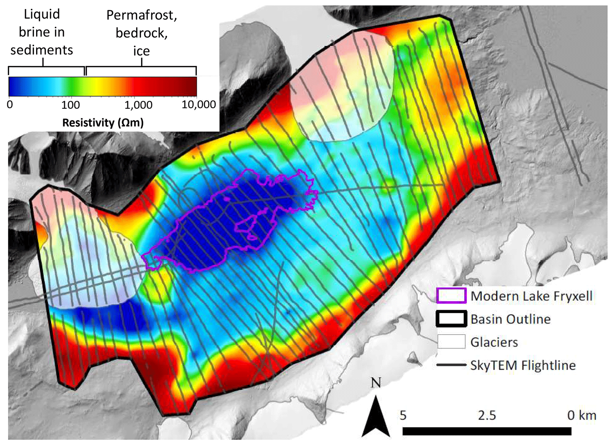
Figure 6Mean resistivity map of constant elevation (−100 m a.s.l., 5 m thick slice) generated from SkyTEM data. Flight lines are shown as a transparent gray, which indicate the flight path of the helicopter as it flew over Fryxell basin in 2011. Each flight line is made up of individual nodes spaced ∼25 m apart. The mean resistivity map was generated in Aarhus Workbench and interpolates between nodes to create a 3D resistivity inversion model. This figure represents just one 5 m thick slice of the 3D inversion taken at 100 m below sea level (in the subsurface). The outline of modern Lake Fryxell is shown in pink and glaciers as transparent polygons. The thick black polygon (basin outline) represents the extent of reliable data, which was truncated at the edge of each flight line to reduce extrapolation artifacts. The digital elevation model (DEM) used for the background (1 m resolution) is from a 2014–15 lidar survey, accessed via OpenTopography (Fountain et al., 2017).
Specialized inversion software, called Aarhus Workbench, was used to process raw resistivity data and invert for layer models of subsurface resistivity (Foley et al., 2016). Mean resistivity maps, which illustrate the mean resistivity of the subsurface at fixed elevation intervals, were generated in Workbench using a spatially constrained (“quasi-3D”) inversion of the data collected from Fryxell basin in 2011 (Viezzoli et al., 2008). These maps are valuable for illustrating lateral continuity and extent of resistivity structures at depth. Slices of constant elevation from 250 to −300 m a.s.l. that are 5 m thick were interpolated to generate mean resistivity maps using a 1000 m search radius and kriging interpolation. Kriging involves the use of a semi-variogram to determine weights during the interpolation, which makes this method well suited to capture spatial correlations. The variogram model used in the kriging interpolation is a simple exponential function with log-transformed resistivity values, a sill value of 0.16, and a range of 1520 m.
Mean resistivity maps were imported into ArcGIS and then overlaid on a digital elevation model (DEM) (Fountain et al., 2017) and high-resolution DigitalGlobe satellite imagery (WorldView-3, provided by the Polar Geospatial Center) to visualize the location and extent of low-resistivity regions. The digital elevation model used for this study was generated from a lidar campaign flown over the McMurdo Dry Valleys in 2015. The digital elevation model has 1 m spatial resolution and covers all of TV (Fountain et al., 2017).
The depth of investigation was determined in Workbench and represents the maximum depth of reliable resistivity models. Regions of low resistivity (<1000 Ω m, typical of lake water and brine-saturated sediments) have a lower depth of investigation (<100 m) due to signal attenuation in conductive materials, whereas regions of high resistivity (>1000 Ω m, typical of ice, permafrost, and bedrock) have a greater depth of investigation (>300 m) because the electromagnetic signal penetrates deeper with less attenuation in these conditions (Christiansen and Auken, 2012; Mikucki et al., 2015; Foley et al., 2016). We are using the threshold of ∼1000 Ω m to broadly distinguish between “high” versus “low” resistivity based on observations from both McGinnis and Jensen (1971) and Mikucki et al. (2015), who broadly define sediments as brine-bearing if they have resistivity from 10 to 1000 Ω m.
Subsurface characteristics and chemistry can be inferred from the relationship of bulk resistivity to temperature, salinity, and liquid volume fraction (Mikucki et al., 2015). Permafrost resistivity varies and can be broken into subgroups depending on degree of saturation and confining properties as described in McGinnis and Jensen (1971). Confining permafrost does not allow any fluid flow, whereas McGinnis and Jensen (1971) define lower-resistivity “aquifrost” as permafrost that allows groundwater flow due to local conditions such as salinity and porosity. Confining layer permafrost tends to have much higher electrical resistivities (<10 000 Ω m) than aquifrosts (50–1000 Ω m) depending on temperature and degree of saturation of the aquifrost (McGinnis and Jensen, 1971).
The regions of low resistivity underlying higher resistivities are interpreted as liquid-brine-saturated sediments capped by permafrost and represent the liquid groundwater extent in Fryxell basin (Mikucki et al., 2015). To calculate the thickness of the permafrost above this briny aquifer, we performed a search from the surface to the first instance at depth of resistivity values at or below a threshold value of 100 Ω m. The 100 Ω m threshold broadly distinguishes between “dry” or hard-frozen permafrost (above 100 Ω m) and aquifrost or unfrozen ground with a significant liquid fraction in pore spaces (Mikucki et al., 2015; Foley et al., 2016). We chose 100 Ω m as our cutoff based on the Dry Valley Drilling Project borehole data comparison in Foley et al. (2016, Fig. 7 therein) that shows resistivity measurements. The borehole DVDP-11 was drilled within our study area, and temperature and salinity were measured within the borehole. These borehole data can be compared to our resistivity profile taken near the borehole site (Foley et al., 2016, Fig. 7 therein). Foley et al. (2016) show a rapid decline in resistivity, from about 100 Ω m down to <5 Ω m, within only 20–30 m. This sharp resistivity gradient corresponds well to an abrupt jump in salinity with depth. Such a salinity increase is consistent with a transition from frozen sediments to liquid brine.
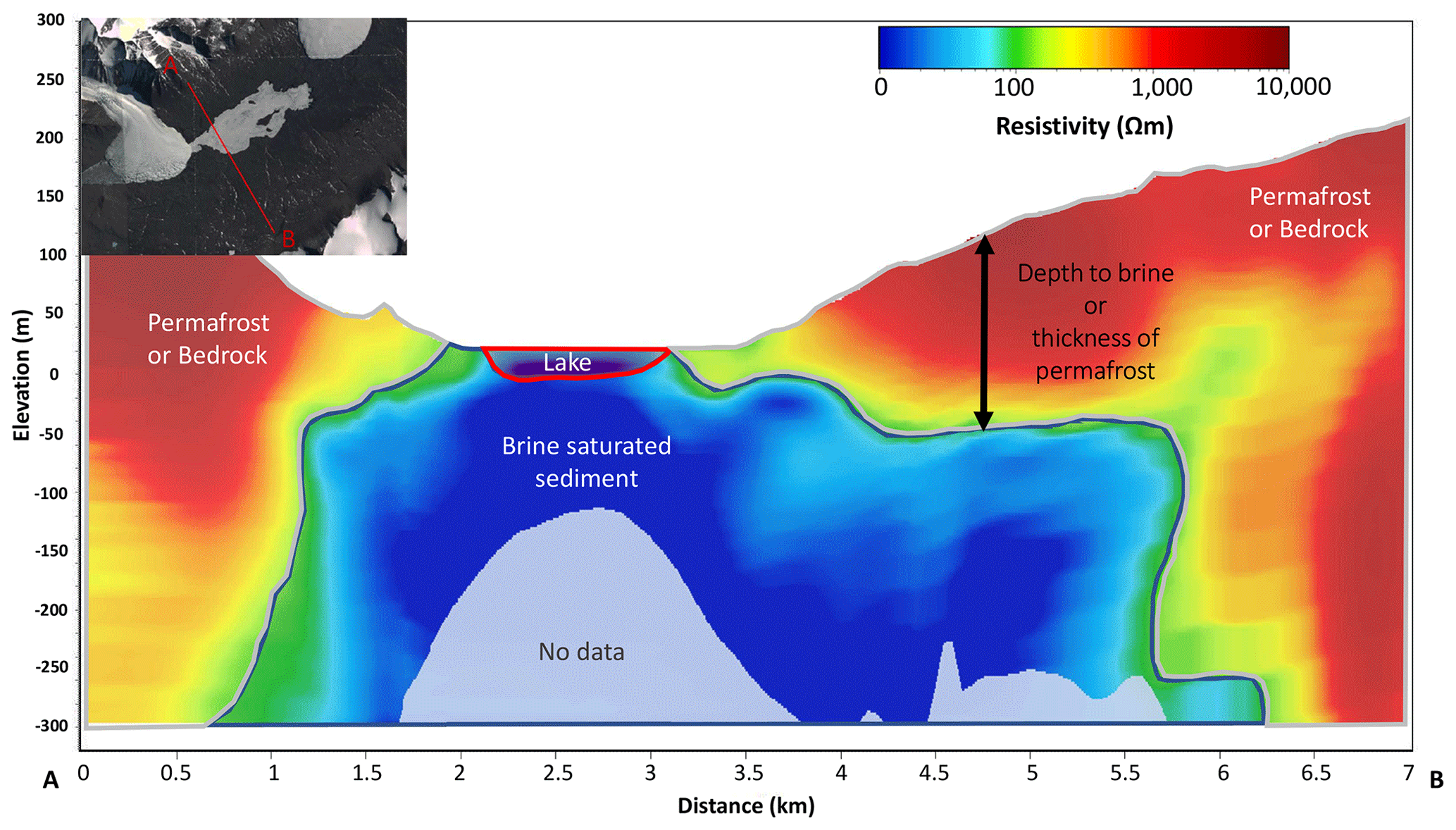
Figure 7North–south transect created from SkyTEM resistivity grid in Workbench. Transect location is shown in inset map (A to B) in upper left corner. Mean resistivity maps were created using a 1 km search radius (2× line spacing) and 5 m elevation slices. Subsurface boundaries are approximated and interpretations based on Mikucki et al. (2015). The subsurface boundary between brine-saturated sediments and permafrost is defined using a resistivity threshold of 100 Ω m.
Workbench was then used to export location, elevation, and depth to brine for each node point of resistivity data collected. Depth-to-brine values for each node were interpolated to map distribution of the permafrost–brine boundary. Depth-to-brine maps were smoothed using a low-pass filter in ArcGIS to reduce noise, which was particularly high around the edges, where data density was lower, and signal-to-noise ratios were less favorable.
2.2 Modeling permafrost thickness and age, analytical model
Permafrost thickness, which is taken as the depth to the 100 Ω m boundary, was used to calculate time since initiation of permafrost freeze-back resulting from lake drainage. We adapted Eq. (5) from Osterkamp and Burn (2003):
where t is the age of permafrost in years, s is a conversion factor from seconds to years, d is the thickness of permafrost (m), Hs is the volumetric latent heat of fusion for sediments corrected for porosity in joules per cubic meter (J m−3), kb is the bulk thermal conductivity of permafrost in watts per meter per kelvin (W m−1 K−1), and Tps is the temperature difference between the atmosphere and permafrost freezing front (K). The average air temperature of Lake Fryxell is −20 ∘C (Obryk et al., 2020), and freezing temperature of brine-saturated sediments is between −5 and −10 ∘C (Foley et al., 2016). Here we use an average brine freezing temperature of −5 ∘C and a maximum brine freezing temperature of −8 ∘C. Therefore, the average Tps is −15 K, and maximum Tps is −12 K. The volumetric latent heat of fusion for sediments corrected for porosity is estimated using Eq. (2):
where Hs is the volumetric latent heat of the sediments, Hv is the volumetric latent heat of water (334 MJ m−3), ϕ is the porosity of the sediment, and ϕa is the fraction of air in pore space. Bulk thermal conductivity of permafrost (kb) is estimated using Eq. (3):
where km is the thermal conductivity of the matrix (Pringle, 2004), kf is the thermal conductivity of the fluid (Engineering Toolbox, 2004), and ka is the thermal conductivity of air (Engineering Toolbox, 2009). All thermal conductivity terms are in units of W m−1 K−1, and values are summarized in Table 1.
Table 1Input values for Eq. (1) through Eq. (4) and Monte Carlo analysis to calculate permafrost ages. Max/min value column shows values within 1 standard deviation resulting in the oldest permafrost ages.
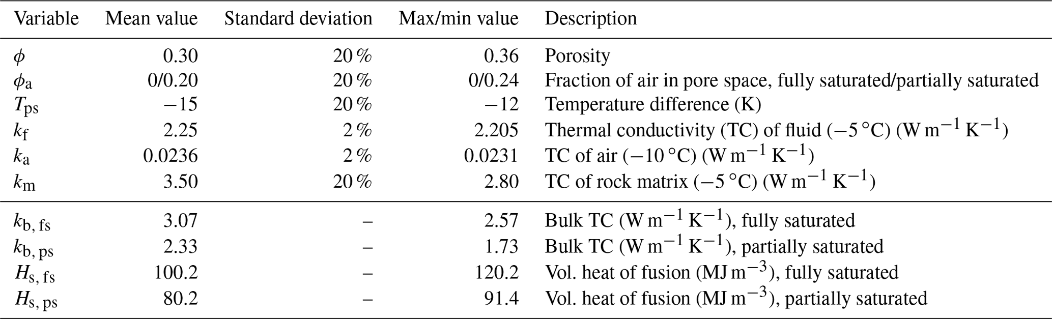
To calculate a range of possible permafrost ages for each elevation, a Monte Carlo statistical analysis was performed. Each input variable was assigned a standard deviation; ϕ, ϕa, Tps, and km were assigned a standard deviation of 20 %, and kf and ka were assigned a standard deviation of 2 % as they are better constrained. We then draw 10 000 realizations, where each input variable is drawn from a normal distribution with mean value and standard deviation as listed in Table 1. For each realization we calculate permafrost age assuming completely saturated sediment (ϕa=0) as well as partially saturated sediment. This approach assumes a normal distribution of all parameters and a homogeneous substrate in both space and time for simplification purposes.
To produce a deterministic upper bound of permafrost ages, Eq. (1) was calculated using the maximum or minimum possible value within 1 standard deviation for each input variable. Hs was maximized by assigning a maximum ϕ (adding 1 standard deviation), with and without air in the pore space. Minimum kb was calculated by minimizing km by subtracting 1 standard deviation and maximizing ϕ by adding 1 standard deviation, with and without air in pore space. Tps was minimized by adding 1 standard deviation from the average value (Table 1).
2.3 Modeling permafrost thickness and age, 1D numerical vertical diffusion model
The model in Sect. 2.2 uses Eq. (1) to calculate permafrost age, assuming a constant Tps through time for simplification; however paleotemperature reconstructions point to a gradual cooling during the Holocene (Steig et al., 2000; Monnin et al., 2004). In order to explore this further, we used a second approach to calculating permafrost ages using a 1D numerical (finite-difference) model, solving the classical Stefan problem of vertical heat diffusion coupled with latent heat release during freezing. The upper boundary condition is a prescribed temperature that is lower than the freezing point of the sub-permafrost brines. Tps can be either held constant during numerical experiments (described in Sect. 2.2) or can be prescribed to vary with time. The bottom boundary condition of the numerical model is a constant heat flux, set to the geothermal flux of 0.080 W m−2, consistent with two borehole-based estimates proximal to the study area (boreholes DVDP-6 and CIROS-1 in Table 1 of Morin et al., 2010). Other model parameters are based on the same permafrost properties listed in Table 1. Existing observational constraints indicate that under modern conditions in the study area, the temperature at the bottom of the permafrost is ca. −10 ∘C (e.g., Foley et al., 2016, Fig. 7 therein), while ground surface temperature is ca. −20 ∘C (Obryk et al., 2020), yielding Tps of about −10 ∘C. We then applied a linear cooling rate of 1, 2, 3, and 4 ∘C over the last 10 000 years to model the cooling trend observed in the Holocene Taylor Dome paleotemperature reconstructions (Steig et al., 2000; Monnin et al., 2004). The ice core constraints appear to be best approximated by the linear cooling trend of 3 ∘C per 10 000 years. The numerically obtained permafrost thickness evolution with time can be fit well (R2=0.9996) with an empirical power relation:
where (like Eq. 1 above) t is the age of permafrost in years, and d is the thickness of permafrost in meters. Note that Eq. (1) can be rewritten in the same power-law form with a time exponent of 0.5 rather than 0.424.
Airborne resistivity data were used to map groundwater and permafrost extent within Fryxell basin. A large low-resistivity region (<100 Ω m) extends hundreds of meters away from the modern lake extent (Figs. 6, 7). The edges of the resistivity map shown in Fig. 6 commonly show a very strong gradient of resistivity, which are mostly artifacts of the interpolation. Defining the interpolation search radius (here we chose 1000 m) is a balance in allowing enough overlap between surrounding model nodes to avoid gaps in the spatial mapping. However, a larger search radius does produce some interpolation artifacts around the edges. The interpolation artifacts are not a concern for regions where data coverage is good (for example, in the center of the map in Fig. 6), and the search radius is interpolating between nodes on all sides. We therefore truncated the maps (shown as black basin outline in Fig. 6) to the edge of the flight lines to remove extrapolation artifacts.
In addition to mapping groundwater, higher resistivities overlaying low-resistivity brine in the valley floor are interpreted as regions of permafrost which range from ∼5 m thick around the lake edge to over 200 m thick higher up on the valley walls (Fig. 7). Permafrost is thinnest near the modern lake edge and increases in thickness with increasing distance from the lake edge (Fig. 8). Permafrost thickness frequency displays a bimodal distribution, with one mode <50 m thick (near lake edge) and another peak around 150 to 200 m, which occurred farther up the valley walls (Fig. 9). Permafrost resistivity varies depending on water content and temperature. Confining permafrost generally had values above 10 000 Ω m, which was only observed in some regions of Fryxell basin (Mikucki et al., 2015; McGinnis and Jensen, 1971). A lower-resistivity permafrost layer (between 100 and 1000 Ω m) extends from the brine layer to approximately 81 m a.s.l. (Fig. 7).
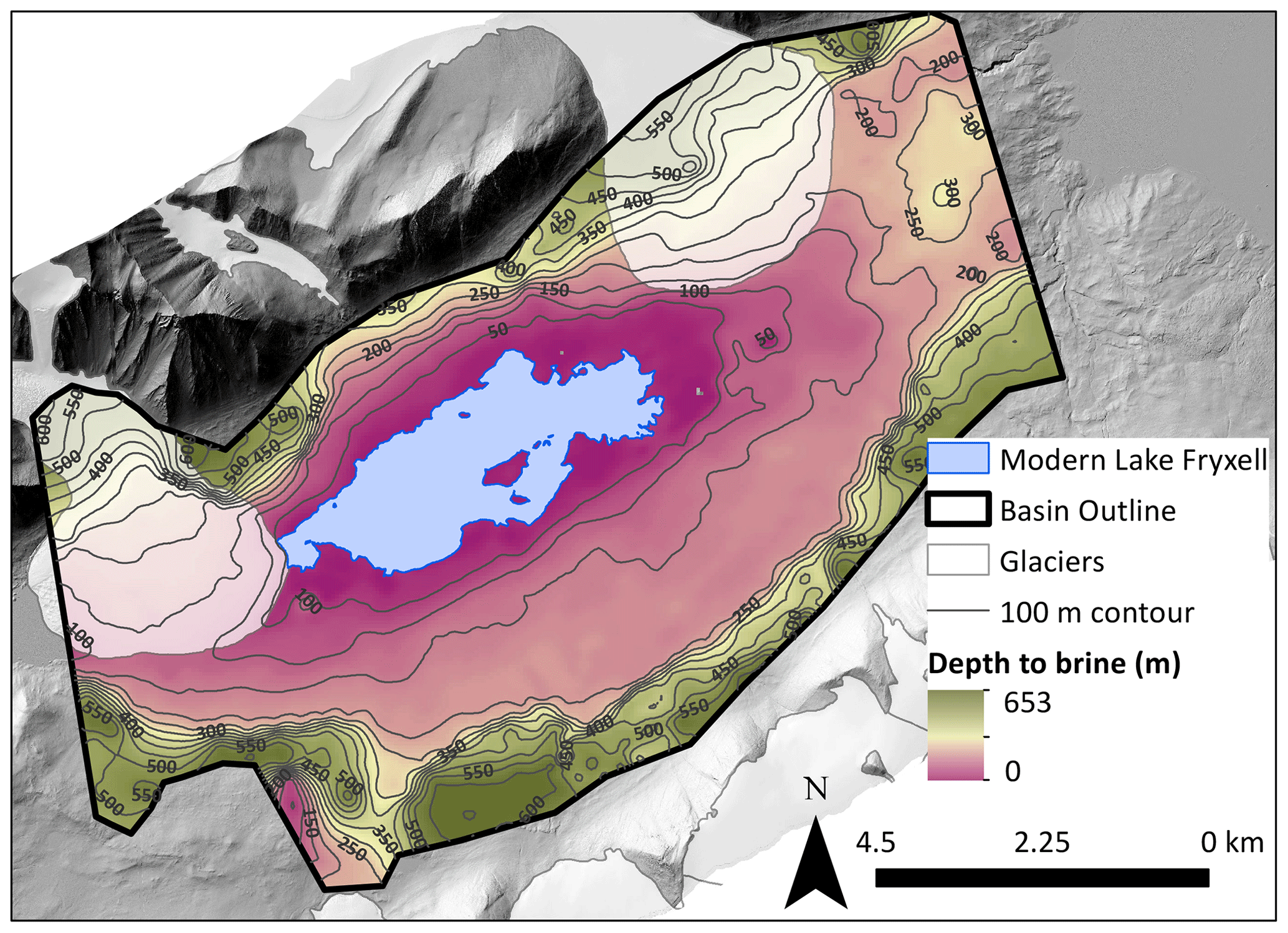
Figure 8Map showing depth to 100 Ω m brine–permafrost boundary generated from SkyTEM data. Interpolation was smoothed using a low-pass filter in ArcGIS to reduce edge noise. Edges (higher elevations and deeper brine layers) are less reliable because of inversion interpolation artifacts and limitations of depth of investigation. The thick black polygon (basin outline) represents the extent of reliable data, which was truncated at the edge of each flight line to reduce extrapolation artifacts. DEM (1 m resolution) is from a 2014–15 lidar survey, accessed via OpenTopography (Fountain et al., 2017).
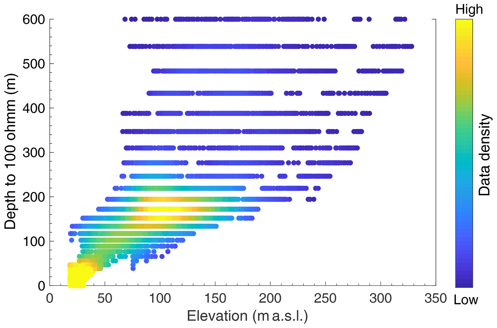
Figure 9Elevation in meters above sea level (m a.s.l.) versus depth to 100 Ω m brine–permafrost boundary in Fryxell basin. Each point represents an individual SkyTEM node (shown as the flight lines in Fig. 6). Data density is displayed as a color ramp, where yellow points indicate higher data density, and blue points indicate lower data density.
Calculated permafrost ages are plotted against ranges of possible porosity, bulk thermal conductivity, and temperature differences (Fig. 10). The effect of a partially saturated versus fully saturated substrate on the volumetric latent heat of fusion for sediments corrected for porosity (Hs) and bulk thermal conductivity (kb) was also investigated (Fig. 10). We assumed partially saturated conditions to yield the oldest possible permafrost ages; however we recognize that assuming a homogeneous partially saturated substrate at this permafrost–brine boundary is an oversimplification.
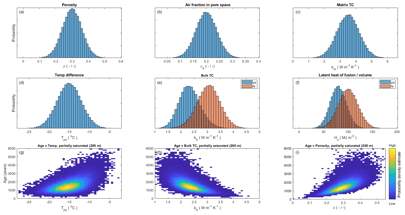
Figure 10Monte Carlo sensitivity analysis of permafrost age inputs; kb and Hs include partially saturated (ps) and fully saturated (fs) substrate conditions. Panels (g)–(i) show how variations in temperature, bulk TC, and porosity affect the age of permafrost. Data density is displayed as a color ramp, where yellow points indicate higher data density, and blue points indicate lower data density.
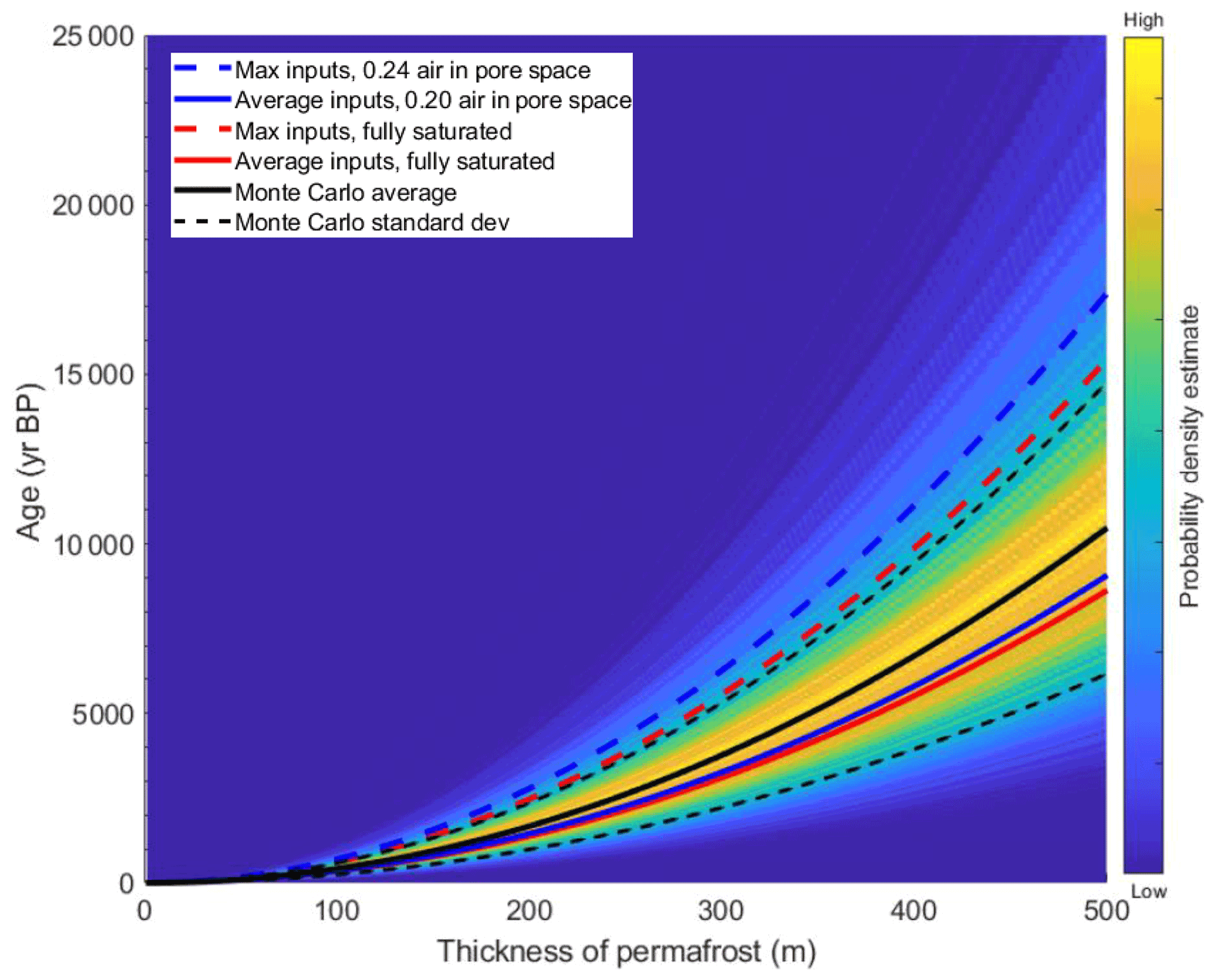
Figure 11Monte Carlo age versus elevation probability for 10 000 iterations of Eq. (1) with average inputs and assigned standard deviation. Monte Carlo average result shown as solid black line and 1 standard deviation as dashed black line. Permafrost ages for average (solid) and maximum inputs (dashed) into Eq. (1), for partially (blue) and completely saturated (red) conditions. Maximum inputs with air fraction in pore space of 0.24 yields maximum possible ages (dashed blue). Data density is displayed as a color ramp, where yellow points indicate higher data density, and blue points indicate lower data density.
Lower depth-to-brine values (thinner permafrost) found at low elevations (<80 m a.s.l.) yielded a smaller range in possible ages. A wide range of calculated ages is seen at higher elevations (>80 m a.s.l.), and therefore the deeper and older permafrost ages are less constrained (Fig. 11). Maximum permafrost ages for partially saturated conditions (0.24 air fraction in pore space) yielded slightly older ages compared to the first-order calculation using average inputs and fully saturated conditions, resulting in a ∼500-year increase in age (approximately 1.5 to 1 ka) for shallow brines between “average” and “maximum” results (Fig. 11). Figure 12 shows the range of possible ages for a discrete depth to brine (permafrost thickness) of 50, 140, and 200 m as calculated from the Monte Carlo analysis for both partially saturated and fully saturated conditions. The age uncertainty is smallest for shallower brines (thinner permafrost) compared to deeper brines (thicker permafrost) (Fig. 12). The middle panel of Fig. 12 shows the age probability distribution for 140 m thick permafrost, which roughly corresponds to the 81 m a.s.l. sill level.
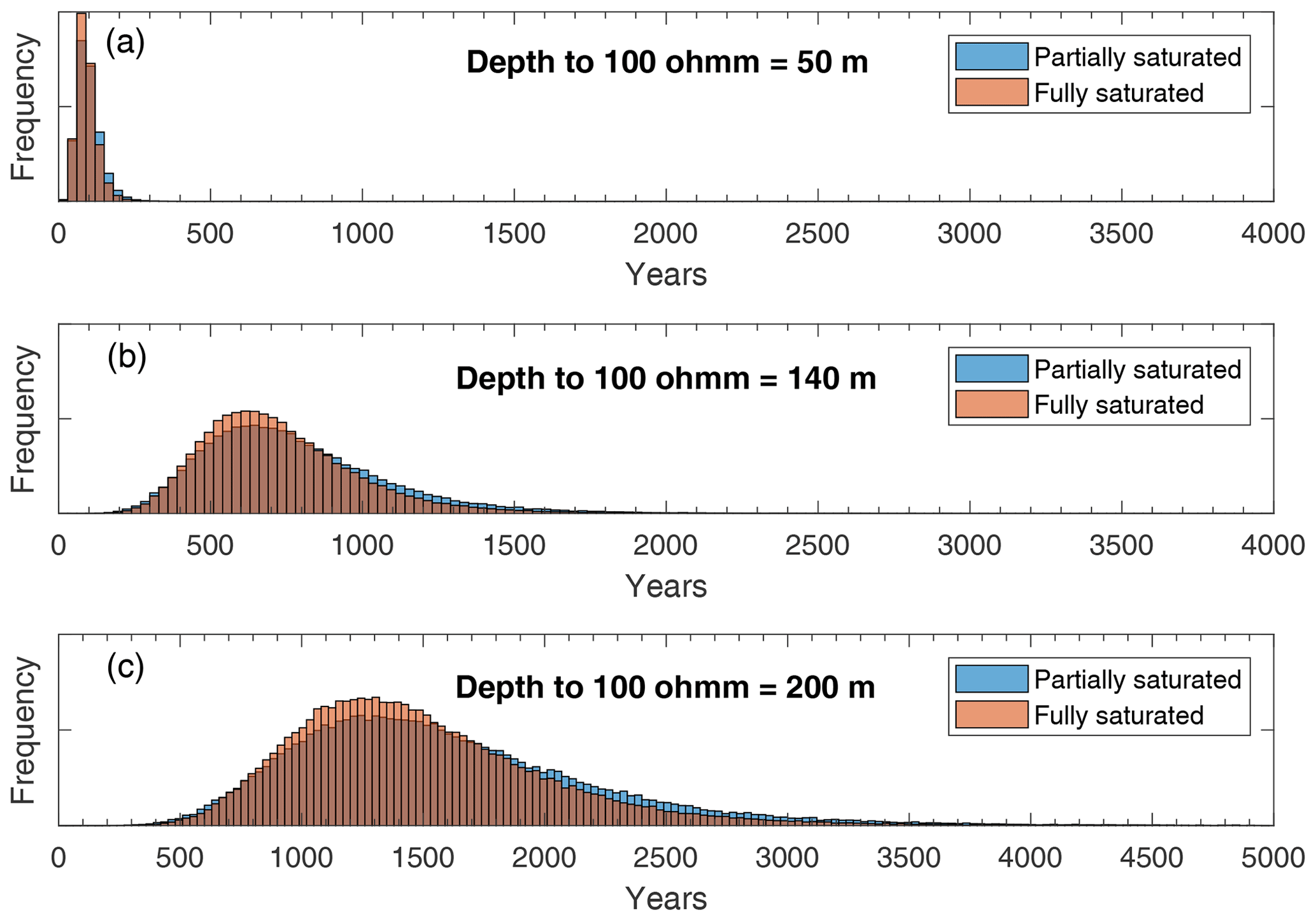
Figure 12Age estimates from Monte Carlo analysis as discrete depth to 100 Ω m brine–permafrost boundary. Each panel shows Monte Carlo analysis results for partially saturated (blue) and fully saturated (orange) conditions at three discrete depths to brine. The shallowest depth to brine (a, 50 m) shows how age of permafrost is relatively well constrained. Thicker depths to brine (b, 140 m or c, 200 m) show how increasing depth to brine also results in less constrained ages of permafrost. A partially saturated substrate (blue bars) results in slightly older permafrost ages compared to a fully saturated (orange bar) substrate.
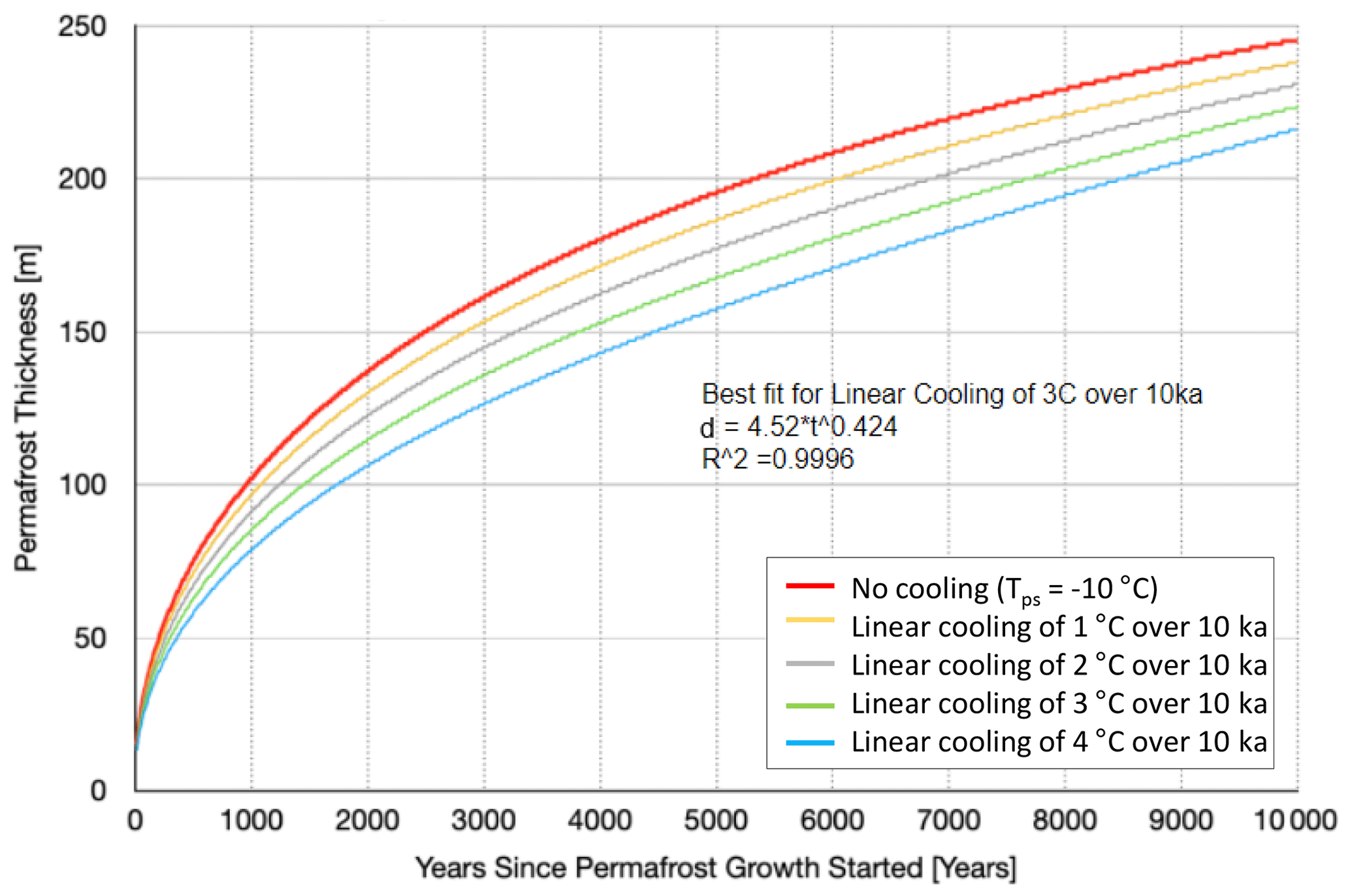
Figure 13Results from 1D numerical (finite-difference) model solving the classical Stefan problem of vertical heat diffusion coupled with latent heat release during freezing. The plot shows how age of permafrost increases with increasing permafrost thickness for various linear cooling trends to simulate lowering temperatures in the Holocene. The equation shown above shows the best fit line for an applied linear cooling rate of 3 ∘C over 10 000 years (green line; Eq. 4).
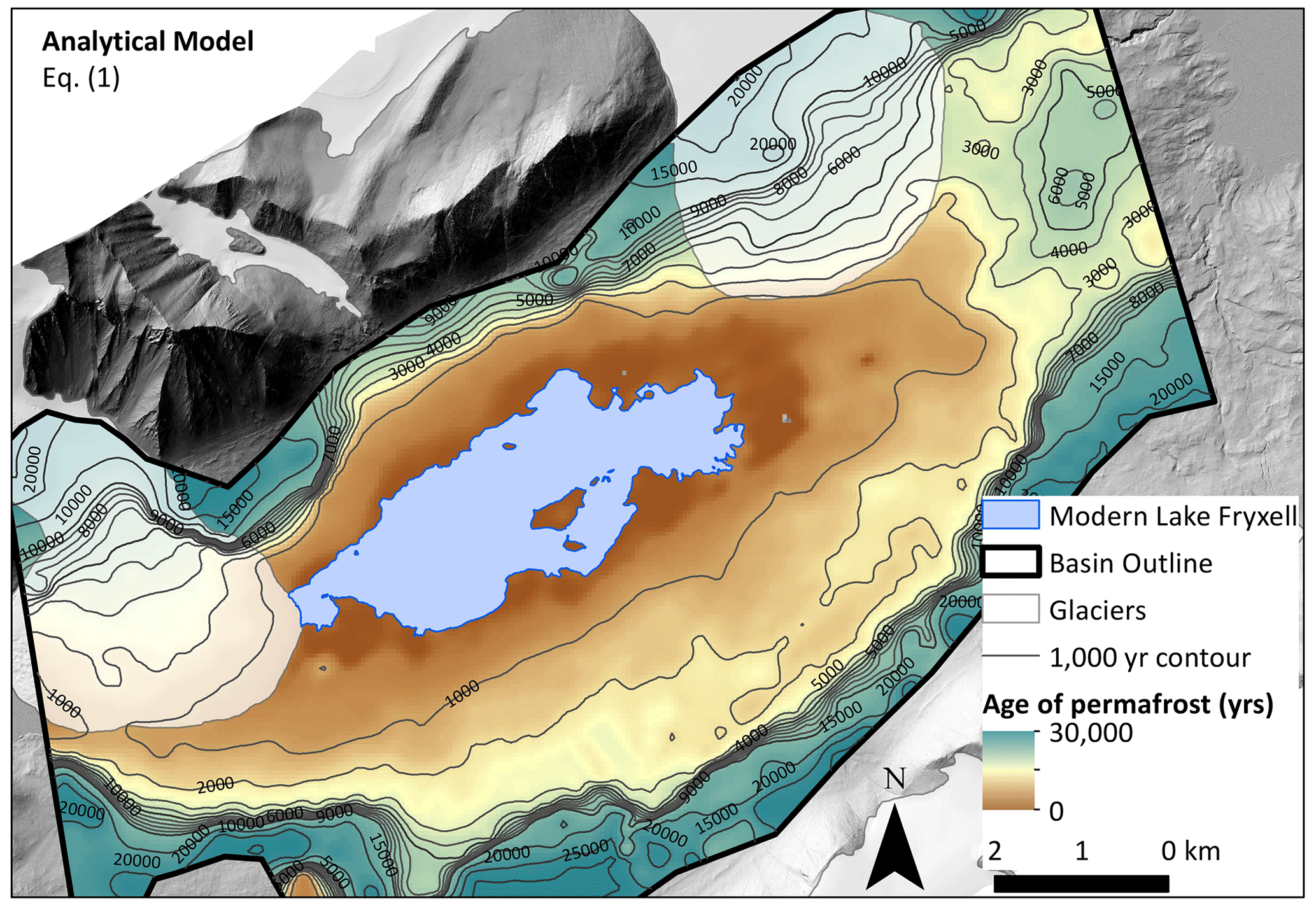
Figure 14Analytical model results of maximum permafrost age distribution in Fryxell basin calculated using Eq. (1) (Osterkamp and Burn, 2003). Age is calculated using depth to permafrost–brine boundary (defined as 100 Ω m). Contours represent age of permafrost in years before present, implying higher lake levels (up to 81 m a.s.l. sill level) during the Late Holocene, ∼1.5 ka. Note that contours switch to 5000-year intervals after 10 000 years. Because of such a large permafrost age gradient at high elevations, the 1000-year contours were illegible. The DEM (1 m resolution) is from a 2014–15 lidar survey, accessed via OpenTopography (Fountain et al., 2017).
Permafrost age was mapped using both methods outlined in Sect. 2.2 and 2.3. First, we mapped permafrost age using the analytical model (using maximum value, partially saturated inputs in Table 1), which calculated permafrost age using depth to brine–permafrost boundary and Eq. (1) (Fig. 14). We then mapped permafrost age using the 1D numerical vertical diffusion model using the best fit (Eq. 4) from Fig. 13 assuming a 3 ∘C linear cooling trend of the last 10 ka (Fig. 15). The age of permafrost was capped at 30 ka in Fig. 15 because this method is not as accurate for very thick permafrost (around the edges of the map), and so this model is best used for younger and thinner permafrost. Both methods produce relatively young permafrost ages around Lake Fryxell; however the model based on 1D numerical vertical diffusion output (Eq. 4) yields slightly older ages.
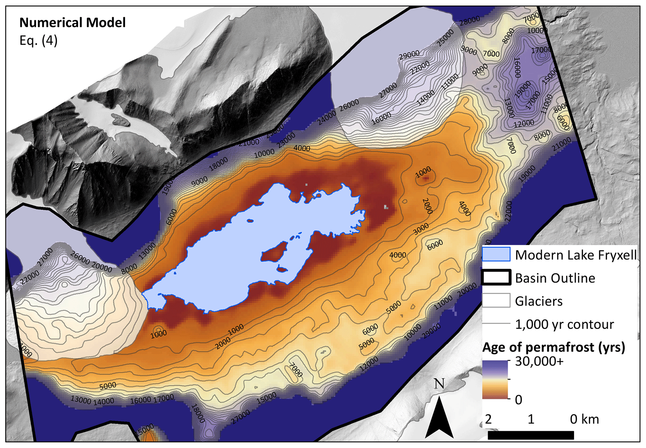
Figure 15Numerical model results of permafrost age distribution in Fryxell basin calculated using Eq. (4). Age is calculated using depth to permafrost–brine boundary (defined as 100 Ω m). Contours represent age of permafrost in years before present, implying higher lake levels (up to 81 m a.s.l. sill level) during the Late Holocene, ∼4 ka, which is older than the results from the analytical model shown in Fig. 14. Note that contours end at 30 000 years BP. Because of such a large permafrost age gradient at high elevations, contours were illegible. The color ramp also stops at 30 000 years BP since the model is not accurate for thick (hence older) permafrost. DEM (1 m resolution) is from a 2014–15 lidar survey, accessed via OpenTopography (Fountain et al., 2017).
Permafrost ages from the two methods were then plotted as a function of sounding point elevation to compare to previously reported 14C and OSL ages at corresponding elevations (Figs. 16, 17). A comparison of all three methods shows that even maximum permafrost age calculations cannot reproduce 14C ages of paleodeltas from Hall and Denton (2000). OSL dates are in rough agreement with permafrost age calculations, especially for low elevations surrounding the modern lake edge (<30 m a.s.l.) (Figs. 16, 17).
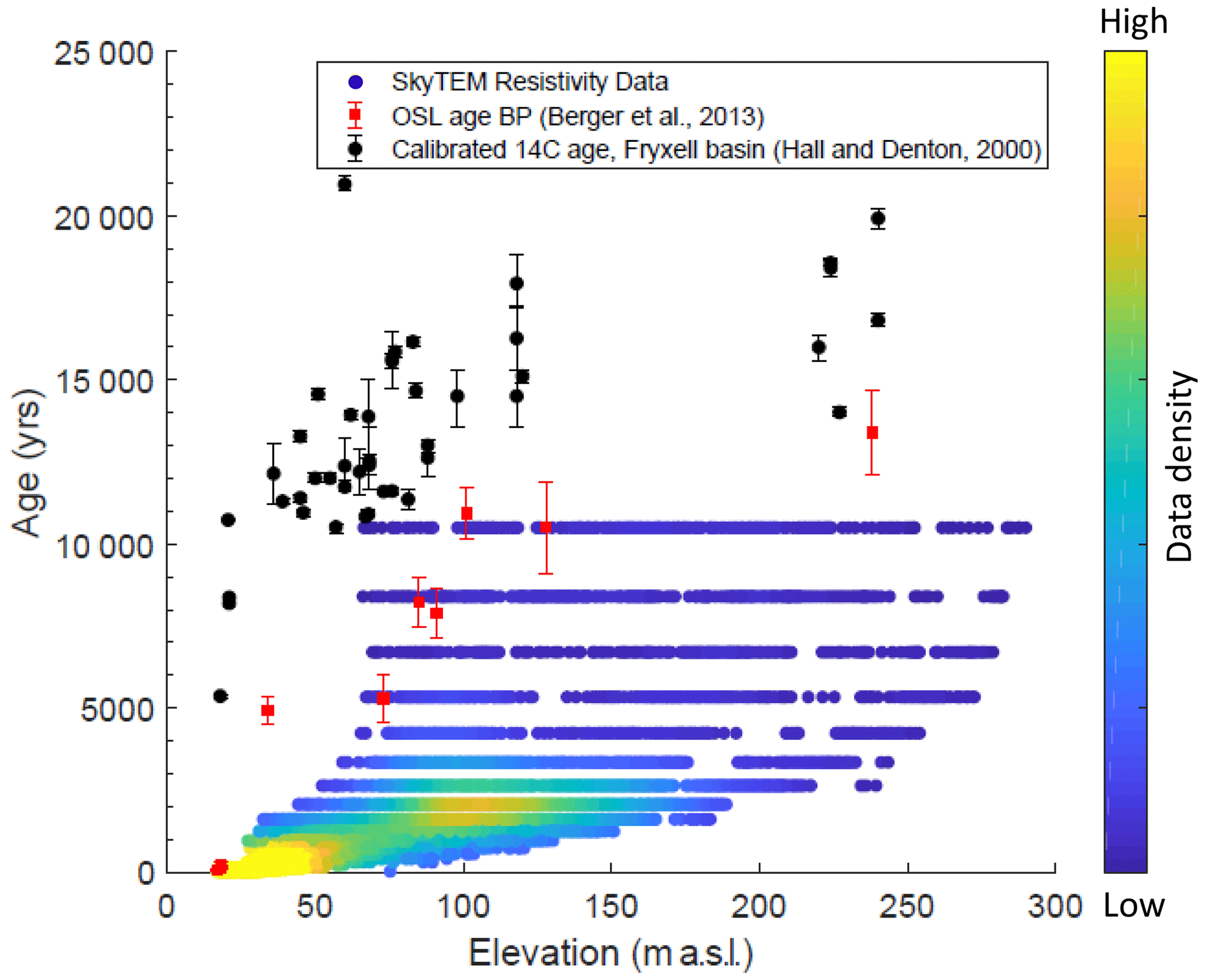
Figure 16Permafrost ages calculated using the analytical model (Eq. 1) applied to SkyTEM resistivity data. Depth to brine (100 Ω m) and inputs from Table 1 were used in Eq. (1) to calculate maximum permafrost age. Permafrost ages are colored by data density, where yellows and greens represent higher data density, and blues represent lower data density. Ages are better constrained for younger, shallower permafrost, so ages were cut off at 400 m depth to brine (corresponding to permafrost ages of ∼11 000 years BP). 14C (Hall and Denton, 2000) and OSL (Berger et al., 2013) ages collected from deltas in Lake Fryxell basin are plotted for comparison.
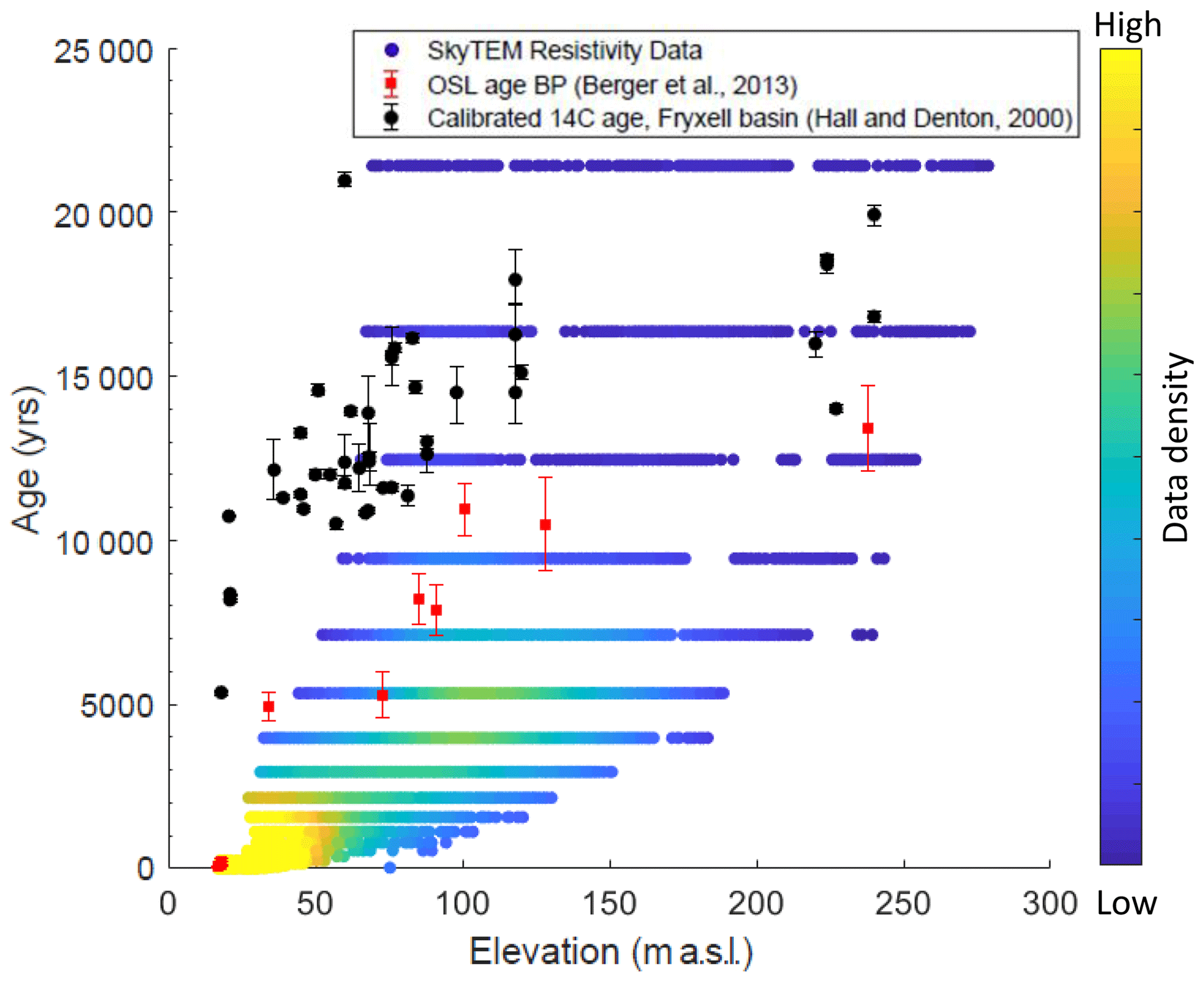
Figure 17Permafrost ages calculated using the numerical model (Eq. 4) applied to SkyTEM resistivity data. Depth to brine (100 Ω m) was used to calculate permafrost age, assuming a 3 ∘C/10 000 years cooling trend over the Late Holocene. Permafrost ages are colored by data density, where yellows and greens represent higher data density, and blues represent lower data density. Ages are better constrained for younger, shallower permafrost, so ages were cut off at 400 m depth to brine (corresponding to permafrost ages of ∼21 000 years BP). 14C (Hall and Denton, 2000) and OSL (Berger et al., 2013) ages collected from deltas in Lake Fryxell basin are plotted for comparison.
In polar regions, ubiquitous permafrost isolates surface water from deeper groundwater systems by forming a relatively impermeable layer. Exceptions occur where large lakes form and have formed in the past. This is because adding a lake and changing lake levels drastically alter the surface thermal boundary conditions from, for example, −20 ∘C (i.e., the typical mean annual air temperature in Taylor Valley; Obryk et al., 2020) when no lake is present to around 0 ∘C when year-round liquid water occupies the surface. Airborne resistivity data revealed a low-resistivity groundwater signal that extends hundreds of meters away from the modern lake edge of Lake Fryxell. In the MDV, this groundwater system is overlaid by permafrost 0 to hundreds of meters thick. We propose that this region of low resistivity beneath higher-resistivity permafrost is a relic thaw bulb from higher lake levels of the past. The presence of a large paleolake would have altered the thermal regime of inundated regions, allowing for a broader groundwater connection throughout much of TV. As the lake level dropped to modern levels, the paleolake bed was exposed to subfreezing surface temperatures, resulting in permafrost growth from the top down. Gradual freeze-back of past lake beds following lake level drop (transient talik) has been observed in the Arctic, and permafrost continues to form until steady-state conditions are reached (Neill et al., 2020).
Permafrost age calculations can be compared to paleotemperature records from Taylor Dome to correlate paleoclimate events with hydrologic responses. Lake levels appear to have been the highest around or after 12 ka (OSL date from ∼250 m a.s.l.), the end of a warming period from 15 to 12 ka (Steig et al., 2000). Lake levels likely remained high from 12 to 8 ka and subsequently dropped due to the retreat of the grounded Ross Ice Shelf from the mouth of TV (Hall and Denton, 2000; Hall et al., 2004; Anderson et al., 2016; Spector et al., 2017). After the removal of the ice dam, lake levels would not be able to exceed the sill level at Coral Ridge (Fig. 1). We measure sill elevation to be 78–81 m a.s.l. based on the digital elevation model of Fountain et al. (2017). Since channel erosion rates are unknown, we use the present-day bank elevation (81 m a.s.l.) as the topographic threshold that defines the boundary of the Lake Fryxell watershed. Any additional hydrologic input into Lake Fryxell above this 81 m a.s.l. level would spill into the McMurdo Sound via the channel that cuts through Coral Ridge (Fig. 1).
During the Late Holocene, a much larger talik would have existed beneath a larger paleolake, and the thickness of permafrost above this relic talik can be used to calculate time since lake drainage. This study uses both an analytical model (Eq. 1) and a numerical model (Eq. 4) to calculate permafrost age. Neither of the two models takes into account the rate of lake level drop, and both model results would be the same if we assume a constant rate of lake level drop or an instantaneous lake level drop. The analytical model assumes constant Tps for simplification; however we explored the scenario of a variable Tps (3 ∘C cooling over 10 000 years) in the numerical model (Eq. 4, Figs. 13 and 15). Lateral heat flux from modern and ancient lakes is not addressed in this study; however it may be important to understand equilibrium thresholds for this evolving groundwater system.
When it comes to analyzing the potential importance of putative lake level variability at elevations <81 m a.s.l., it is important to note in our Fig. 9 that the cluster of thin permafrost at low elevations occurs for elevations <50 m a.s.l., where permafrost is estimated to be <50 m thick. Comparatively few of our estimates of permafrost thickness fall between 50 and 140 m, with corresponding surface elevations between 50 and 81 m a.s.l. The only other high-abundance cluster of permafrost thickness is 140–200 m, with corresponding surface elevations between 81 and 150 m a.s.l. This cluster represents the lake levels that occurred when the ice dam was still present. When the ice dam is not present, the hydrology of Fryxell basin favors lake levels that are considerably lower than the sill level of 81 m a.s.l. and that reach mostly up to ca. 50 m a.s.l., which corresponds to the other cluster of common permafrost thicknesses that are <50 m thick.
Permafrost age calculations indicate Late Holocene lake level high stands (up to ∼81 m a.s.l., 63 m higher than modern Lake Fryxell) from roughly 1.5 ka (Fig. 14) to 4 ka (Fig. 15) that would have filled both Lake Fryxell and Lake Hoare basins (Fig. 3b). Permafrost ages span a wide range of elevations because the depth-to-brine boundary only roughly follows surface topography (Figs. 16, 17). This is probably an indication of subsurface heterogeneity (bedrock, till, lacustrine sediment, and buried ice distribution), which is also apparent in resistivity maps. Shallower depth-to-brine values (younger ages) are better constrained compared to older and higher-elevation brines, as suggested by Monte Carlo statistical analysis, and can be used as an estimate of uncertainty (Figs. 11, 12). For this reason, we are not using this method to necessarily date the timing of the highest lake levels. This paper discusses GLW in the context of past lake level high stands; however other methods are likely better at determining very old lake levels compared to this method of using resistivity data.
Application of a linear cooling of 3 ∘C in the last 10 000 years to a numerical model of permafrost growth (Eq. 4) still yields fairly young ages for elevations below the 81 m a.s.l. sill level (<150 m thick permafrost results in ∼4 ka; green line below). This would be about 2.5 ka older than our original approach using the analytical solution (Eq. 1) (Osterkamp and Burn, 2003). Even though the results vary between the two methods, the data still suggest that a larger lake occupied Fryxell basin between 1.5 ka (analytical method) and 4 ka (1D vertical diffusion model explained above). At higher elevations with permafrost thicknesses ≥200 m we obtain ages between 7–8 ka.
Using two methods to calculate permafrost ages from resistivity data, it was still not possible to yield ages for lake occupation that fully agreed with those estimated by 14C ages of delta deposits (Hall and Denton, 2000) (Figs. 16, 17). Radiocarbon dating from Hall and Denton (2000) suggests that lake levels were higher than modern between 22 to 5 ka. OSL dates (Berger et al., 2013) estimate past lake level high stands to be more recent, existing between 12–5 ka. Neither OSL nor 14C suggests lake level high stands younger than 5 ka. Our permafrost age calculations agree more with the OSL chronology than the 14C at all elevations (Figs. 16, 17), but both chronologies have their limitations. OSL records the burial age of the quartz grain, which may be different from the deposition age. Rates of past sediment transport and deposition are not currently known, so this lag in deposition versus burial time is unresolved. Secondly, OSL dates are collected from some depth below the surface, meaning the dates may not be an accurate representation of the most recent occupation of that delta or lake level elevation (this will also be true for 14C samples collected away from the surface). Several studies have shown a substantial radiocarbon reservoir effect in the MDVs, but modern lake edges and streams have been shown to be mostly well equilibrated with the modern atmosphere (e.g., Doran et al., 1999; Hendy and Hall, 2006). Doran et al. (2014) did note some exceptions. In fact, out of four moat microbial mat samples dated (all in <1 m of water), only one was equilibrated with the modern atmosphere. The others carried 14C ages of 2324±96, 9334±71, and 2608±48 years BP. So clearly, even in modern lakes it is possible for lake edge material to carry a significant carbon reservoir. A large glacial lake of the past may have had even more ancient unequilibrated carbon associated with it due to melt coming from the ancient Ross Ice Shelf without the opportunity for significant equalization with the atmosphere (e.g., through direct subaqueous glacial melt and moats being more closed to the atmosphere). Moreover, under climates colder than today lake ice may have been thicker and 14C equilibration with ambient atmosphere more restricted. Levy et al. (2017) point out that 14C have consistently produced dates 5–10 ka older than OSL samples from the same locations in Garwood Valley.
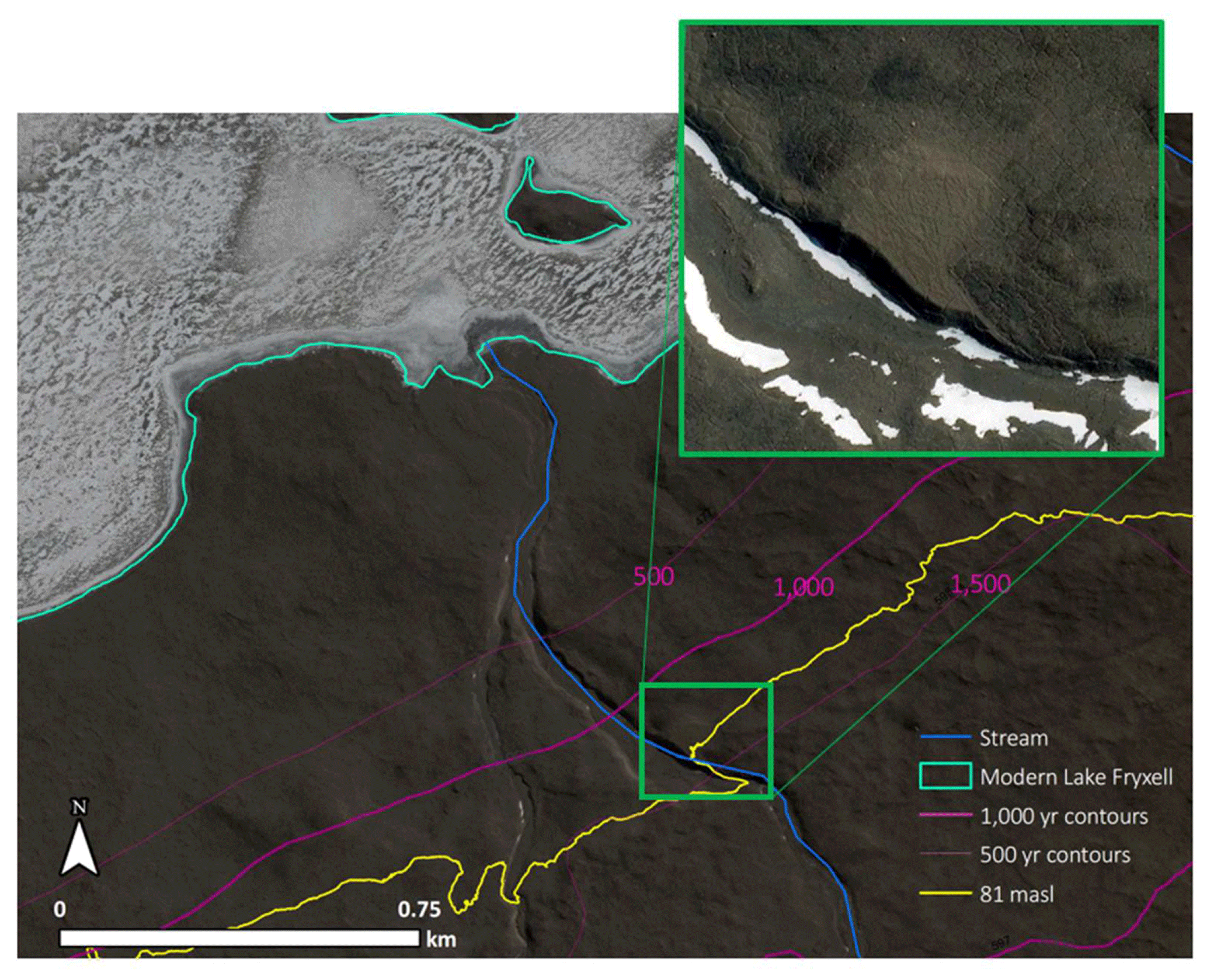
Figure 18Maximum permafrost ages calculated using the analytical model (Eq. 1) are shown as pink contours and indicate roughly 1.5 ka permafrost at 81 m a.s.l. (yellow elevation contour). An extremely well-preserved delta on Crescent Stream is located at roughly 81 m a.s.l. and shown in inset map (green box). Image © 2017 DigitalGlobe, Inc. provided by the Polar Geospatial Center.
Multiple lines of evidence support our permafrost age calculation. Permafrost at approximately 81 m a.s.l. dates at 4 and 1.5 ka using the numerical and analytical models, respectively. During this time, Taylor Dome ice core records show a highly variable Holocene climate with temperatures up to 5 ∘C above modern until 1–2 ka, when temperatures came down to modern levels (Steig et al., 2000; Monnin et al., 2004). Multiple studies in the MDVs make a direct connection with air temperatures and hydrologic response (Obryk et al., 2017; Doran et al., 2008, 2002b), which supports a potential connection between higher lake levels during the relatively warm Holocene. Also, at roughly the sill level (∼81 m a.s.l.), there is a large and very well-preserved delta on Crescent Stream in Fryxell basin, with nearly zero slope and sharp transitions between the topset and foreset, suggesting low degrees of weathering (Fig. 18). Weathering of delta deposits has not been rigorously addressed in previous literature, and we cannot quantify the relationship between delta appearance with age because there are many unknown variables (i.e., deposition rate, geology, duration of lake occupation, and erosion rate); however, through visual comparison in the field as well as using DEMs and satellite imagery, the delta on Crescent Stream is the most well-defined delta in Fryxell basin. Because this delta occurs at 81 m a.s.l., the maximum possible lake level without grounded ice at the mouth of TV, the delta may have formed through multiple cycles of filling and drainages. Lake Fryxell could have reached 81 m a.s.l. multiple times in the past, and we suggest that periods with warmer-than-modern conditions such as the Late Holocene could result in this common lake level elevation, and any additional hydrologic input would result in spillover into the McMurdo Sound. The combination of a highly preserved delta deposit at 81 m a.s.l., the approximate permafrost age of 1.5 to 4 ka, and warmer-than-modern temperatures in the Late Holocene suggests that it was possible for lake level to be at the sill level sometime in the last few thousand years. This is somewhat at odds with previous studies that have shown evidence for drawdown events (significantly lower than modern) between 1–4 ka (Lyons et al., 1998) or at 6.4, 4.7, 3.8, and 1.6 ka (Whittaker et al., 2008). A partial desiccation event or events in the Late Holocene cannot be resolved using either paleodelta age or resistivity data from this study.
Lake levels in TV have fluctuated in the past, leaving behind a complex history of overprinted lacustrine deposits and subsurface thermal signatures. A novel approach using airborne transient electromagnetic surveys provides new evidence that supports the existence of much higher lake levels in Fryxell basin by constraining lake level timing and extent. This study provides new insight on lake level evolution in TV during the Holocene, a period in which past studies are contradictory, and significant gaps remain. Lake levels were higher potentially during and after the LGM, when an ice dam blocked the mouth of TV, allowing for lake levels to increase by over 280 m compared to modern levels. Taylor Dome ice core records indicate an abrupt warming of >15 ∘C from 15–12 ka, (Steig et al., 2000), which may have coincided with the maximum lake level of GLW. Following ice sheet retreat approximately 8 ka, GLW drained, and lake level likely fluctuated from at or below modern levels (18 m a.s.l.) up to 81 m a.s.l. between 8 and 1.5 ka. Around 4–1.5 ka, lake levels were at the 81 m a.s.l. sill level and have subsequently dropped to or below modern levels. Our chronology of Fryxell basin lake level history based on modeling of the thermal legacy of the lake is better supported by previously published OSL ages than 14C ages of paleodeltas on the valley walls.
Small changes in climate such as a 5 ∘C higher temperature in the Late Holocene (Monnin et al., 2004) could have sustained up to 60 m higher lake levels in Fryxell basin. Closed-basin MDV lakes are characterized by high variability and extreme sensitivity to both climate and geologic drivers. Modern and paleohydrologic evidence indicates a highly dynamic system in which modest temperature forcings can initiate a large-scale hydrologic response.
Lake level data for Fig. 5 are available at https://mcm.lternet.edu/content/lake-level-surveys-mcmurdo-dry-valleys-antarctica-1991-present (last access: 16 July 2020, Doran and Gooseff, 2020).
SkyTEM data collected in 2011 are available at https://doi.org/10.15784/601071 (Tulaczyk, 2017).
KFM wrote the text, conducted data analysis, and made the figures. PTD and SMT helped write the text as well as develop methods and concepts. SMT and NTF provided the conceptual framework for the paper including the method to determine permafrost age from Osterkamp and Burns (2003) and from numerical modeling. EA, TSB, NF, and DG provided technical details and support regarding electromagnetic data and processing as well as edits to the text. TSB also provided help on Monte Carlo simulations. HAD, JAM, and RAV all contributed to SkyTEM data collection, the conceptual framework for the project, and edits to the text and figures.
The authors declare that they have no conflict of interest.
Any opinions, findings, conclusions, or recommendations expressed in
the material are those of the authors and do not necessarily reflect the
views of the National Science Foundation.
Publisher's note: Copernicus Publications remains neutral with regard to jurisdictional claims in published maps and institutional affiliations.
We would like to thank the two reviewers as well as the editors of The Cryosphere for their excellent suggestions, which greatly improved the manuscript.
This research is funded by the National Science Foundation (NSF) grant no. OPP-1637708 as part of the Long-Term Ecological Research program. This material is based upon work supported by the NSF Graduate Research Fellowship under grant no. 1247192. Support for Krista F. Myers and Peter T. Doran was also provided by the Louisiana State University John Franks Chair Fund. Contributions of Slawek M. Tulaczyk and Neil T. Foley to this work were supported by two grants from the NSF (grant nos. 1344349 and 1644187). Contributions of Jill A. Mikucki were supported by NSF grant no. OPP-1344348. Contributions for Ross A. Virginia were supported by NSF grant no. 1043618. Other support for this project was provided by NSF grant nos. 1643687, 1643536, and 1643775. Geospatial support for this work was provided by the Polar Geospatial Center under NSF-OPP awards 1043681 and 1559691.
This paper was edited by Elizabeth Bagshaw and reviewed by Stefano Nerozzi and one anonymous referee.
Anderson, J. B., Conway, H., Bart, P. J., Witus, A. E., Greenwood, S. L., McKay, R. M., Hall, B. L., Ackert, R. P., Licht, K., Jakobsson, M., and Stone, J. O.: Ross Sea paleo-ice sheet drainage and deglacial history during and since the LGM, Quaternary Sci. Rev., 100, 31–54, 2014.
Anderson, J. B., Wilson, G. S., Fink, D., Lilly, K., Levy, R. H., and Townsend, D.: Reconciling marine and terrestrial evidence for post LGM ice sheet retreat in southern McMurdo Sound, Antarctica, Quaternary Sci. Rev., 157, 1–13, 2016.
Arcone, S. A., Delaney, A. J., Prentice, M. L., and Horsman, J. L.: GPR reflection profiles of sedimentary deposits in lower Taylor Valley, Antarctica, paper presented at Twelfth International Conference on Ground Penetrating Radar, 15–19 June, Birmingham, United Kingdom, 2008.
Berger, G. W., Doran, P. T., and Thomsen, K. J.: Micro-hole and multigrain quartz luminescence dating of Paleodeltas at Lake Fryxell, McMurdo Dry Valleys (Antarctica), and relevance for lake history, Quat. Geochronol., 18, 119–134, 2013.
Chinn, T. J. H.: Accelerated Ablation at a Glacier Ice-Cliff Margin, Dry Valleys, Antarctica, INSTAAR, Univ. Color., 19, 71–80, 1987.
Christiansen, A. V. and Auken, E.: A global measure for depth of investigation, Geophysics, 77, 4, WB171–WB177, 2012.
Cunningham, W. L., Leventer, A., Andrews, J. T., Jennings, A. E., and Licht, K. J.: Late Pleistocene-Holocene marine conditions in the Ross Sea, Antarctica: Evidence from the diatom record, Holocene, 9, 129–139, 1999.
Denton, G. H. and Marchant, D. R.: The Geologic Basis for a Reconstruction of a Grounded Ice Sheet in McMurdo Sound, Antarctica, at the Last Glacial Maximum, Geogr. Ann. Ser. A, Phys. Geogr., 82, 167–211, 2000.
Doran, P. T. and Gooseff, M. N.: McMurdo Dry Valleys LTER: Lake level surveys in the McMurdo Dry Valleys, Antarctica from 1991 to present, Environmental Data Initiative, https://doi.org/10.6073/pasta/3d0e0c4d844792d9964dd4179a3d 83aa, 2020.
Doran, P. T., Berger, G. W., Lyons, W. B., Wharton, R. A., Divisson, M. L., Southon, J., and Dibb, J. E.: Dating Quaternary lacustrine sediments in the McMurdo Dry Valleys, Antarctica, Palaeogeogr. Palaeocl., 147, 223–239, 1999.
Doran, P. T., McKay, C. P., Clow, G. D., Dana, G. L., Fountain, A. G., Nylen, T., and Lyons, W. B.: Valley floor climate observations from the McMurdo dry valleys, Antarctica, 1986–2000, J. Geophys. Res.-Atmos., 107, 1–12, 2002a.
Doran, P. T., Priscu, J. C., Lyons, W. B., Walsh, J. E., Fountain, A. G., McKnight, D. M., Moorhead, D. L., Virginia, R. A., Wall, D. H., Clow, G. D., and Fritsen, C. H.: Antarctic climate cooling and terrestrial ecosystem response, Nature, 415, 517–520, 2002b.
Doran, P. T., McKay, C. P., Fountain, A. G., Nylen, T., McKnight, D. M., Jaros, C., and Barret, J. E.: Hydrologic response to extreme warm and cold summers in the McMurdo Dry Valleys, East Antarctica, Antarct. Sci. 20, 499–509, 2008.
Doran, P. T., Kenig, F., Lawson Knoepfle, J., Mikucki, J. A., and Lyons, W. B.: Radiocarbon distribution and the effect of legacy in lakes of the McMurdo Dry Valleys, Antarctica, Limnol. Oceanogr., 59, 811–826, 2014.
Dugan, H., Obryk, M., and Doran, P. T.: Lake ice ablation rates from permanently ice-covered Antarctic lakes, J. Glaciol., 59, 491–498, 2013.
Engineering ToolBox: Ice – Thermal Properties, available at: https://www.engineeringtoolbox.com/ice-thermal-properties-d_576.html (last access: 20 February 2020), 2004.
Engineering ToolBox: Air – Thermal Conductivity, available at: https://www.engineeringtoolbox.com/air-properties-viscosity-conductivity-heat-capacity-d_1509.html (last access: 20 February 2020), 2009.
Foley, N., Tulaczyk, S., Auken, E., Schamper, C., Dugan, H., Mikucki, J., Virginia, R., and Doran, P.: Helicopter-borne transient electromagnetics in high-latitude environments: An application in the McMurdo Dry Valleys, Antarctica, Geophysics, 81, WA87–WA99, 2016.
Foley, N., Tulaczyk, S. M., Grombacher, D., Doran, P. T., Mikucki, J., Myers, K. F., Foged, N., Dugan, H., Auken, E., and Virginia, R.: Evidence for Pathways of Concentrated Submarine Groundwater Discharge in East Antarctica from Helicopter-Borne Electrical Resistivity Measurements, Hydrology, 6, 54, 2019.
Fountain, A. G., Nylen, T. H., Monaghan, A., Basagic, H. J., and Bromwich, D.: Snow in the McMurdo Dry Valleys, Antarctica, Int. J. Climatol., 30, 633–642, 2010.
Fountain, A. G., Saba, G., Adams, B., Doran, P., Fraser, W., Gooseff, M., Obryk, M., Priscu, J. C., Stammerjohn, S., and Virginia, R. A.: The Impact of a Large-Scale Climate Event on Antarctic Ecosystem Processes, Bioscience, 66, 848–863, 2016.
Fountain, A. G., Fernandez-Diaz, J. C., Obryk, M., Levy, J., Gooseff, M., Van Horn, D. J., Morin, P., and Shrestha, R.: High-resolution elevation mapping of the McMurdo Dry Valleys, Antarctica, and surrounding regions, Earth Syst. Sci. Data, 9, 435–443, https://doi.org/10.5194/essd-9-435-2017, 2017.
Gooseff, M. N., Barrett, J. E., Adams, B. J., Doran, P. T., Fountain, A. G., Lyons, W. B., McKnight, D. M., Priscu, J. P., Sokol, E. R., Takacs-Vesbach, C., Vandegehuchte, M. L., Virginia, R. A., and Wall, D. H.: Decadal ecosystem response to an anomalous melt season in a polar desert in Antarctica, Nat. Ecol. Evol., 1, 1334–1338, 2017.
Hall, B. L. and Denton, G. H.: Radiocarbon chronology of Ross Sea drift, eastern Taylor Valley, Antarctica; evidence for a grounded ice sheet in the Ross Sea at the last glacial maximum, Geogr. Ann. Ser. A Phys. Geogr., 82, 305–336, 2000.
Hall, B. L., Baroni, C., and Denton, G. H.: Holocene relative sea-level history of the Southern Victoria Land Coast, Antarctica, Glob. Planet. Change, 42, 241–263, 2004.
Hall, B. L., Hoelzel, A. R., Baroni, C., Denton, G. H., LeBoeuf, B. J., Overturf, B., and Topf, A. L.: Holocene elephant seal distribution implies warmer-than-present climate in the Ross Sea, P. Natl. Acad. Sci. USA, 103, 10213–10217, 2006.
Hall, B. L., Denton, G. H., Stone, J. O., and Conway, H.: History of the grounded ice sheet in the Ross Sea sector of Antarctica during the Last Glacial Maximum and the last termination, Antarctic palaeoenvironments and earth-surface processes, 381, 167–181, 2013.
Hall, B. L., Denton, G. H., Heath, S. L., Jackson, M. S., and Koffman, T. N. B.: Accumulation and marine forcing of ice dynamics in the western Ross Sea during the last deglaciation: Supplementary Info, Nat. Geosci., 8, 625–628, 2015.
Hendy, C. H. and Hall, B. L.: The radiocarbon reservoir effect in proglacial lakes: Examples from Antarctica, Earth Planet. Sc. Lett., 241, 413–421, 2006.
Horsman, J. L.: The origin of sandy terraces in eastern Taylor Valley, Antarctica, from Ground Penetrating Radar: A test of the Glacial Lake Washburn delta interpretation, MS thesis, 258 pp., Plymouth State University, Plymouth, New Hampshire, 2007.
Lawrence, J. P., Doran, P. T., Winslow, L. A., and Priscu, J. C.: Subglacial brine flow and wind-induced internal waves in Lake Bonney, Antarctica, Antarct. Sci., 32, 223–237, 2020.
Levy, J.: How big are the McMurdo Dry Valleys? Estimating ice-free area using Landsat image data, Antarct. Sci., 25, 119–120, 2013.
Levy, J. S., Rittenour, T. M., Fountain, A. G., and O'Connor, J. E.: Luminescence dating of paleolake deltas and glacial deposits in Garwood Valley, Antarctica: Implications for climate, Ross ice sheet dynamics, and paleolake duration, Bull. Geol. Soc. Am., 1289, 1071–1084, 2017.
Lyons, W. B., Tyler, S. W., Wharton, R. A., McKnight, D. M., and Vaughn, B. H.: A Late Holocene desiccation of Lake Hoare and Lake Fryxell, McMurdo Dry Valleys, Antarctica, Antarct. Sci., 10, 247–256, 1998.
Lyons, W. B., Fountain, A., Doran, P. T., Priscu, J. C., Neumann, K., and Welch, K. A.: Importance of landscape position and legacy: The evolution of the lakes in Taylor Valley, Antarctica, Freshw. Biol., 43, 355–367, 2000.
McGinnis, L. D. and Jensen, T. E.: Permafrost-Hydrogeologic Regimen in Two Ice-Free Valleys, Antarctica, from Electrical Depth Soundings, Quaternary Res., 1, 389–409, 1971.
Mikucki, J. A., Auken, E., Tulaczyk, S., Virginia, R. A., Schamper, C., Sorensen, K. I., Doran, P. T., Dugan, H., and Foley, N.: Deep groundwater and potential subsurface habitats beneath an Antarctic dry valley, Nat. Commun., 6, 1–9, 2015.
Monnin, E., Steig, E., Siegenthaler, U., Kawamura, K., Schwander, J., Stauffer, B., Stocker, T., Morse, D., Barnola, J., Bellier, B., Raynaud, D., and Fischer, H.: Evidence for substantial accumulation rate variability in Antarctica during the Holocene, through synchronization of CO2 in the Taylor Dome, Dome C and DML ice cores, Earth Planet. Sc. Lett., 224, 45–54, 2004.
Morin, R. H., Williams, T., Henrys, S. A., Magens, D., Niessen, F., and Hansaraj, D.: Heat Flow and Hydrologic Characteristics at the AND-1B borehold, ANDRILL McMurdo Ice Shelf Project, Antarctica, Geosphere, 6, 370–378, 2010.
Neill, H., Roy-Leveille, P., Lebedeva, L., and Ling, F.: Recent advances (2010–2019) in the study of taliks, Permafrost Periglac., 31, 346–357, 2020.
Obryk, M. K., Doran, P. T., Waddington, E. D., and McKay, C. P.: The influence of föhn winds on Glacial Lake Washburn and palaeotemperatures in the McMurdo Dry Valleys, Antarctica, during the Last Glacial Maximum, Antarct. Sci., 29, 457–467, 2017.
Obryk, M. K., Doran, P. T., Fountain, A. G., Myers, M., and McKay, C. P.: Climate from the McMurdo Dry Valleys, Antarctica, 1986–2017: Surface Air Temperature Trends and Redefined Summer Season, J. Geophys. Res.-Atmos., 125, e2019JD032180, https://doi.org/10.1029/2019JD032180, 2020.
Osterkamp, T. E. and Burn, C. R.: Permafrost, in: Encyclopedia of Atmospheric Sciences, edited by: Holton, J. R., Academic, Oxford, UK, 1717–1729, 2003.
Pringle, D. J.: Thermal Conductivity of Sea Ice and Antarctic Permafrost, Thesis, available at: http://researcharchive.vuw.ac.nz/xmlui/handle/10063/313 (last access: 3 August 2020), 2004.
Sørensen, K. I. and Auken, E.: SkyTEM – A new high-resolution helicopter transient electromagnetic system, Explor. Geophys., 35, 191–199, 2004.
Scott, R. F.: The Voyage of the “Discovery”, C. Scribner's Sons, New York, 1905.
Spector, P., Stone, J., Cowdery, S. G., Hall, B., Conway, H., and Bromley, G.: Rapid early-Holocene deglaciation in the Ross Sea, Antarctica, Geophys. Res. Lett. 44, 7817–7825, 2017.
Steig, E. J., Morse, D. L., Waddington, E. D., Stuiver, M., Grootes, P. M., Mayewski, P. A., Twickler, M. S., and Whitlow, S. I.: Wisconsinan and Holocene Climate History from an Ice Core at Taylor Dome, Western Ross Embayment, Antarctica, Geogr. Ann. Ser. A Phys. Geogr., 82A, 213–235, 2000.
Stuiver, M., Reimer, P. J., and Reimer, R. W.: CALIB 7.1, available at: http://calib.org, last access: 4 June 2018.
Toner, J. D., Sletten, R. S., and Prentice, M. L.: Soluble salt accumulations in Taylor Valley, Antarctica: Implications for paleolakes and Ross Sea Ice Sheet dynamics, J. Geophys. Res.-Earth Surf., 118, 198–215, 2013.
Toner, J. D., Catling, D. C., and Sletten, R. S.: The geochemistry of Don Juan Pond: Evidence for a deep groundwater flow system in Wright Valley, Antarctica, Earth Planet. Sci. Lett., 474, 190–197, 2017.
Tulaczyk, S.: 2011 Time-domain ElectroMagnetics data for McMurdo Dry Valleys [data set], U.S. Antarctic Program (USAP) Data Center, https://doi.org/10.15784/601071, 2017.
Viezzoli, A., Christiansen, A. V., Auken, E., and Sørensen, K. I.: Quasi-3D modelling of airborne TEM data by Spatially Constrained Inversion, Geophysics, 73, F105–F113, 2008.
Ward, S. H. and Hohmann, G. W.: Electromagnetic theory for geophysical applications, in: Electromagnetic methods in applied geophysics: SEG, edited by: Nabighian, M. N., Society of Exploration Geophysicists, 130–311, https://doi.org/10.1190/1.9781560802631.ch4, 1988.
Whittaker, T., Hall, B., Hendy, C., and Spaulding, S.: Holocene depositional environments and surface-level changes at Lake Fryxell, Antarctica, Holocene, 18, 775–786, 2008.