By Andy May
In my last post, on Scafetta’s new millennial temperature reconstruction, I included the following sentence that caused a lot of controversy and discussion in the comments:
“The model shown uses a computed anthropogenic input based on the CMIP5 models, but while they use an assumed climate sensitivity to CO2 (ECS) of ~3°C, Scafetta uses 1.5°C/2xCO2 to accommodate his estimate of natural forcings.”
I thought in the context of the post, the meaning was clear. But, Nick Stokes, and others, thought I meant that ECS was an input parameter to the CMIP5 climate models. This is not true, ECS is computed from the model output. If you pull the above quote out of the post and view it in isolation, it can be interpreted that way, so I changed it to the following which is unambiguous on the point.
“The model shown uses a computed anthropogenic input based on the CMIP5 models, but while they use an assumed climate sensitivity to CO2 (ECS computed from the CMIP5 ensemble model mean) of ~3°C, Scafetta uses 1.5°C/2xCO2 to accommodate his estimate of natural forcings.”
Then we received criticism about the computation of the ensemble model mean ECS, some said the IPCC did not compute an ensemble mean of ECS. This is nonsense, they compute it in AR5 (IPCC, 2013, p. 818). A portion of the table is shown below as Figure 1.

Figure 1. A portion of IPCC AR5 WG1 Table 9.5, page 818. The average ECS of the CMIP5 models is shown at the bottom as 3.2 degrees.
As you can see in Figure 2, most of the models greatly overestimate warming in the mid to upper tropical troposphere. A pressure of 300 hPa occurs at about 30,000 feet or 10 km altitude and 200 hPa is at about 38,000 feet or 12 km altitude. The top of the troposphere is the tropopause, and in the tropics, it is usually between 150 hPa or 14 km and 70 hPa or 18 km.

Figure 2. CMIP5 models versus weather balloon observations in green in the mid- to upper troposphere. The details of why the models fail statistically can be seen in a 2018 paper by McKitrick and Christy here. All model runs shown use historical forcing to 2006 and RCP 4.5 after then.
The purple line in Figure 2 that tracks the weather balloon observations (heavy green line), is the Russian INM-CM4 model. As we can see, INM-CM4 is the only model that matches the weather balloon observations reasonably well, yet it is an outlier among the other CMIP5 models. Because it is an outlier, it is often ignored. In Figure 1 we can see that if ECS is computed from the INM-CM4 output, we get 2.1°C/2xCO2 (degrees warming due to doubling the CO2 concentration). Yet, while an ECS of 2.1 is clearly matching observations since 1979, the model average is 3.2. It is significant, literally, that INM-CM4 is one of the few models that passes the statistical test used in McKitrick and Christy, 2018 (see their Table 2). This is why I used the word “assumed.” The evidence clearly says 2.1, so 3.2 must be assumed. ECS is not an input to the models, but tuning the models changes ECS and the modelers closely watch the value when tuning their models (Wyser, Noije, Yang, Hardenberg, & Declan O’Donnell, 2020).
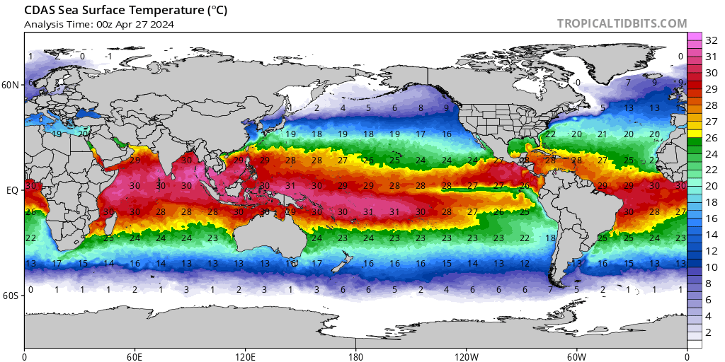
McKitrick and Christy chose the tropical middle to upper troposphere for their comparison very carefully and deliberately (McKitrick & Christy, 2018). This part of the atmosphere is sometimes called the tropospheric “hot spot” (See Figure 3). Basic physics and the IPCC climate models suggest that, if greenhouse gases (GHGs) are causing the atmosphere to warm, this part of the atmosphere should warm faster than the surface. Dr. William Happer has estimated that the rate of lower to middle tropospheric warming should be about 1.2 times the warming at the surface.

The reason is simple. If GHGs are causing the surface to warm, evaporation will increase on the ocean surface. Evaporation and convection are the main mechanism for cooling the surface because the lower atmosphere is nearly opaque to most infrared radiation. The evaporated water vapor carries a lot of latent heat with it as it rises in the atmosphere. The water vapor must rise because it has a lower density than dry air.
As it rises through the lower atmosphere, the air cools and eventually it reaches a height where it condenses to liquid water or ice (the local cloud height). This causes a tremendous release of infrared radiation, some of this radiation warms the surrounding air and some goes to outer space. It is this release of “heat” that is supposed to warm the middle troposphere. Does the “hot spot” exist? Theory says it should, if GHGs are warming the surface significantly. But proof has been elusive. In Figure 4 we plot the surface temperature from the ERA5 weather reanalysis versus the reanalysis temperature at 300 mb (also 300 hPa or about 10 km). The curves below are for most of the globe, the data is from the KNMI climate explorer. I tend to trust reanalysis data, after all it is created after the fact and compared to thousands of observations around the globe. This plot is one example, you can make others easily on the site.
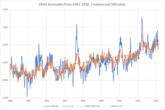
Figure 4. ERA5 weather reanalysis temperatures from the surface (2 meters) in orange and at 300 mbar (10 km). We expect a faster rate of warming at 300 mbar than at the surface, but, instead, the rates are almost the same, with the surface rate slightly higher. The El Niños have a higher rate at 300 mbar, which makes sense.
Surface ocean warming should cause a “hot spot.” We see this in every El Niño in Figure 4. Surface warming due to GHGs should do the same thing, but this is not seen in Figure 4. As I stated above, the models have been tuned to produce an assumed ECS.
Discussion
As a former petrophysical computer modeler, I’m surprised that CMIP5 and the IPCC average results from different models. This is very odd. Standard practice is to examine the results from several models and compare them to observations, this is what John Christy has done in Figure 2. Other comparisons are possible, but his is carefully done to highlight the differences. The spread in model results is huge, some go off scale in 2010. This is not a dataset one should average.
When I was a computer modeler, we would choose one model that appeared to be the best and average multiple runs from just that model. We never averaged runs from different models, it makes no sense. They are incompatible. I still think choosing one model is the “best practice.” I’ve not seen an explanation for why the CMIP5 produces an “ensemble mean.” It seems to be an admission that they have no idea what is going on, if they did they would choose the best model. I suspect it is a political solution for a scientific problem.
Also, the results (see Figures 1 and 2) suggest that the models are out of phase with one another. Figure 2 is a pile of spaghetti. Since it is obvious that natural variability is cyclical (see (Wyatt & Curry, 2014), (Scafetta, 2021), (Scafetta, 2013), and Javier’s posts here and here), this odd practice of averaging out-of-phase model results completely wipes out natural variability and makes it appear nature plays no role in climate. Once you do that, you have no valid way of computing the human impact. They have designed a method that guarantees the computation of a large ECS. Sad.
Works Cited
IPCC. (2013). In T. Stocker, D. Qin, G.-K. Plattner, M. Tignor, S. Allen, J. Boschung, . . . P. Midgley, Climate Change 2013: The Physical Science Basis. Contribution of Working Group I to the Fifth Assessment Report of the Intergovernmental Panel on Climate Change. Cambridge: Cambridge University Press. Retrieved from https://www.ipcc.ch/pdf/assessment-report/ar5/wg1/WG1AR5_SPM_FINAL.pdf
McKitrick, R. & Christy, J., 2018, A Test of the Tropical 200- to 300-hPa Warming Rate in Climate Models, Earth and Space Science, 5:9, p. 529-536
Scafetta, N. (2021, January 17). Climate Dynamics. Retrieved from https://doi.org/10.1007/s00382-021-05626-x
Scafetta, N. 2013, “Discussion on climate oscillations: CMIP5 general circulation models versus a semi-empirical harmonic model based on astronomical cycles, Earth-Science Reviews, 126(321-357).
Wyatt, M., & Curry, J. (2014, May). Role for Eurasian Arctic shelf sea ice in a secularly varying hemispheric climate signal during the 20th century. Climate Dynamics, 42(9-10), 2763-2782. Retrieved from https://link.springer.com/article/10.1007/s00382-013-1950-2#page-1
Wyser, K., Noije, T. v., Yang, S., Hardenberg, J. v., & Declan O’Donnell, a. R. (2020). On the increased climate sensitivity in the EC-Earth model from CMIP5 to CMIP6. Geosci. Model Dev., 13, 3465-3474.
Oh I’ll tell you the problem!
http://phzoe.com/2021/02/06/greenhouse-gases-are-coolants/
This is what I was taught back in the stone age (’50s) when CO2 was 280 ppm. Such numbers you never forget.
Temperature is regulated through pressure by gravity anyway, the real question is the original reason for putting thermometers at airports… increasing the temperature over a runway decreases the air density without any meaningful change in pressure… it literally maintains the same amount of energy per volume. How much does the density change affect the specific heat of a cubic centimeter of air per calorie input?
All the pseudoscience done by the IPCC morons assumed a fixed mass per volume. They can’t even pass grade school science class.
Zoe, go away with your click bait.
Hans in this case Zoe is correct. CO2 will not cause warming. It can’t.
Using standard physics information there are about 1.07E16 CO2 molecules in a cubic meter of air. Using Planck constant a m^3 of air has about .0001 J caused by CO2 emissions.
This warming people speak of is not mentioned in specific heat tables, the Shomate equation, nor the NIST data sheet of CO2.
The forcing equation is BS as it neglects the increased mass of the carbon atoms.
“… tuning the models changes ECS and the modelers closely watch the value when tuning their models.”
and, tuning to expectation = pseudoscience = Cargo-cult science.
GCMs are Cargo-cult science, as in, “Those finicky cargo planes will start landing if we can just get our runway layout just right. Send more money so we can keep making the adjustments.”
They average it out because it is a consensus science, not empirical.
Settled science 😉
Biden goes full on Solyndra.. https://www.google.com/amp/s/qz.com/1968184/biden-could-prove-the-solyndra-scandal-wasnt-a-failure/amp/
Oh, good grief!
“ Eichacker says. “The costs of climate change are incomprehensibly large [and] the downside of losing on a few more Solyndras pales in comparison to not trying to do more.” In other words, better to suffer through a Solyndra than miss out on a Tesla.”
This is the problem now. Leftist driving energy policy 🙁
Yes, the cost of changing the weather is incomprehensibly large.
I still can’t work on what would be wrong with “missing out on a Tesla”. There’s little remarkable with one more electric cart which will inevitably need fossil fuels to keep it on the road.
All EV’s need fossil fuels to keep them on the road
Exactly. Be heck of alot cheaper to buy & putter around in a little electric golf cart if that’s what you feel compelled to do.
Just get the government OUT of venture capitalism. Let those who want to risk their capital risk it, and reap the success or failure from their ventures. This is NO place for government!
It astounds me why so many people don’t understand that simple idea. If people want to risk their, good luck to them. I just don’twant government to risk my money.
A major part of the problem is the large number of people who can’t conceive of ANYTHING being done without government involvement.
The ‘Nanny State’ is an illusion, though, but an illusion that an indoctrinated public believes is giving them value for their money. The reality is; they just make themselves and their friends wealthier while letting the cities turn into shit-holes. Socialism has been a failure everywhere and in every way it has been tried.
This is a very sanitized and spun version of the Solyndra debacle that blames the China boogieman—the real causes were the idiotic module design that doomed the idea on the drawing board and the technical incompetence of the DoE program managers who thought it had a chance of success.
“I suspect it is a political solution for a scientific problem.”
It is that for sure, but also follow the money. Once someone like the IPCC chooses the winner, everybody else can pack it up and go home. Do you know how much money climate scientists and universities/colleges/ngo’s will lose when this happens? Ain’t going to happen. Besides the fact that it is an automatic propaganda winner to have multiple “models” all showing somewhat the same thing.
When I hear the meme, “Follow the money,” I can’t help but think of Hunter Biden and the old joke that “Cocaine is God’s way of telling you that you have too much money.”
As for Andy’s question about, why does IPCC average and ensemble of models that all (or most are clearly) wrong? He does touch on the fact this is political solution, a solution of inclusion. And by including all international players (model teams) who play along with the scam, it gains political support from team’s governments wanting to look like they are “following science.” This is done to garner a “consensus” and to wave it in front of ignorant reporters and politicians, and thus dupe the public with pseudoscience, as the shakedown continues.
Consensus is the realm of politics and religion, of which climate change is both. Climate modeling and by extension most of climate science that seeks to calculate an ECS with that crap is just simply junk science through and through.
The CMIP process IS consensus science at work. Nothing more.
And as the late Michael Crichton said, “If it’s consensus, it’s not science. If it’s science, it’s not consensus.”
Since the IPCC was designed as political solution to provide the rationale for imposing climate policies and making it look like science.
One could just as easily get out one’s deluxe box of coloured pencils and draw a series of squiggles, between 0C and two temperature extremes (say 1.5C and 4.5C) over the next 30 to 40 years and call it science. It would be indistinguishable and just as accurate as the GCM generated image.
Just as inaccurate as the …
My point was: if random scribbles produced with a box of coloured pencils are indistinguishable from the methodical output of state of the art climate models, what does that say about their scientific value, never mind their predictive value?
The question I have is why do they get away with showing actual temperature history compared to the spaghetti chart which include all the RCPs. We are clearly no where near any of the RCP scenarios where GHGs are significantly reduced; we are on and have been on, RCP8.5, and so says the National Academy of Sciences.
Tom, The model runs in Figure 2 use historical forcing to 2006 and RCP 4.5 after 2006. I’ve changed the caption to reflect that.
Edward Norton Lorenz (May 23, 1917 – April 16, 2008) was an American mathematician and meteorologist who established the theoretical basis of weather and climate predictability, as well as the basis for computer-aided atmospheric physics and meteorology.
He discovered that the climate is a chaotic system. That means it is so sensitive to initial conditions that it can’t meaningfully be predicted. Given that, and given that nobody has refuted his observation, why do people continue to write climate models in the conventional manner?
Shhhhhh, stop interfering with sciency talk by recalling facts.
Follow the money.
He discovered that weather is chaotic. The climate of a region not so much.
Evidence?
I would have thought it was self evident.
So, Loy-dumb HAS NO EVIDENCE……
AS ALWAYS
You “would” have thought…… but you are NOT CAPABLE OF IT.
Translation: Loydo has no evidence but can’t bring himself to admit it.
That’s always the sign that you’re about to get something wildly wrong … you “thought”. The only “self evident” thing here is your ignorance.
So self-evident you can’t actually produce any?
Exactly, commieBob, always ask the neo-marxists questions. They hate that because they never have rational answers.
Another Loy-dumb zero-evidence fairy-tale.
How pointless and totally irrelevant.
I read your comments here for a long time, and your comments show me, that you contradict yourself, because your local head climate seems to be very chaotic. 😀
SCNR
Climate is the integral of weather., i.e. the temperature profile. If weather is chaotic then so is the climate.
Mr. do: “He discovered that weather is chaotic. The climate of a region not so much.”
I’ve read elsewhere that climate of a region is basically thirty years of weather, averaged. So take chaos, average it, and you… what… lose the chaos??!! So you take chaotic, random numbers between 2 and 12, average them and you may get 7. This does NOT mean every throw thereafter comes up 7. Play craps and find out the hard way.
“Climate is a coupled, non-linear, chaotic system” (IPCC). Climate is regional, by definition.
You’ve got some ‘splaining to do, son. Please forward your falsifications of Lorenz.
You’ve got to be careful what you define your regions as being. North Dakota, Kansas and Oklahoma are all part of the central plains region but have vastly different climates. Look at the agricultural “growing regions” or growing season maps and you’ll get a lot better definitions of climate regions, at least in the US. Kansas City and Lincoln are pretty close together but have big differences in their heating and cooling degree-days. Yet St Paul and Denver are quite distant with very similar cooling and heating degree days.
Considering climate to be local has always seemed to work for me.
That was supposed to be my point, such as it was. I was alluding to my high school definition of climate (60+ years ago) … “climate is the average weather at a particular location over time.” In my province we have numerous climates, from West Coast Marine to Mediterranean, Alpine, Tundra, Taiga and so on. Each has its own particular set of causes. Trying to pretend there could be some average climate for British Columbia is just silly. Applying the that standard to the whole planet makes a mockery of global “climate change” as a concept.
Thanks for the clarification. I agree with you 100%
Reasons! That’s why.
Post modern science don’t need no logic.
“…don’t need no stinkin’ logic…
So that’s why climate Scientologists call their work projections AKA soothsaying
The spaghetti graph does resemble goat entrails.
Andy, very nice follow up post. My complements.
A key question you implicitly raise is how does Russian climate model INM-CM4 differ from the rest in order to track observations?
I am going from memory of a long analysis of that question by Ron Klutz of Canada (his blog is IIRC Science Matters) some years ago.
These comments may allow newer WUWT readers to focus on the BIG climate model issues, and research for themselves the papers and data underlying them.
As just one example taken from the Climate chapter of TAOT, Andrew Dessler’s second paper in 2010 purported to find positive cloud feedback by comparing clear sky to all sky satellite TOA IR. This was promptly amplified by NASA on their website. The fundamental problem is, his data is an almost perfect shotgun pattern with an r^2 of 0.02. NOTHING—NO TREND. And he should have known that from the gitgo if he had any stats competence at all. That paper arguably comprises academic misconduct.
And as icing on this somewhat mathematical cake, IF you assume cloud feedback is 0, and that WVF is half of explicit AR4 ( which was 2.4 from 1.2) because of the rainfall discrepancy, and then you plug that net net Bode ~0.25 into Lindzen’s curve based on zero feedback 1.2C ECS, then ECS is ~1.6. Which is what Lewis and Curry concluded as the most likely estimate in their series of energy budget method ECS papers. QED.
Thanks Rud. Good analysis. How did we find ourselves in the position of having to prove the alarmists are wrong. We believe that climate is controlled by nature, that is the default position! Now we have to prove human’s do not control the climate, the sci-fi position. Weird.
It has roots in the sociopolitical complex and uncivil rights, where there is a presumption of guilt until proven otherwise. A profitable model that has, surprising many, transferred to science.
You are trying to prove the shaman’s visions are not reality. Has that ever worked for anyone, anywhere, at any time?
Climate alarmism has turned science upside down.
Yes, a good analysis.
Andy, would you have a link to a higher resolution copy of fig.2? I looked on the linked paper in your piece but couldn’t see it.
Thanks.
Alastair, click on Figure 2 and it will appear in full resolution.
Thanks Andy but either I or my computer (or both) must be pretty dumb…clicking on the image (in Firefox) only gets me a 45Mb copy and it’s hard to read the model numbers on the right. Is there a better way? Or am I doing something wrong…or is 45Mb full resolution?
The mysteries of the internet. I can’t click on it either, ususally you can. Try this link:
Click on the image above, that should show it in full resolution.
Thanks for this but it is still only 112Kb and still a bit hard to read the model names. However, many thanks for your private message with the best solution.
The INM model is much more realistic with ocean warm pool temperature:
http://climexp.knmi.nl/data/icmip5_tas_Amon_inmcm4_rcp85_160-179E_-5-5N_n_+++.png
It gets up to 302K in the Nino4 region. It is low now and needs to be at the set point of 30C to be correct.
By contrast, the GISS model achieves the physically impossible:
http://climexp.knmi.nl/data/icmip5_tas_Amon_GISS-E2-H_p3_rcp85_160-179E_-5-5N_n_+++.png
With the tropical warm pool reaching 307K. That is something that cannot occur on planet Earth in the hundred years or next hundred million.
Just to compare with reality, albeit over a shorter time frame:
http://climexp.knmi.nl/data/itao_sst_160-179E_-5-5N_n.png
It is quite clear the temperature gets controlled at 30C. Some overshoot but the regulation is quite tight.
Real time data from 0N, 156E when it was in the warm pool shows just how well the thermostat works.
This stable 30C figure stems from the temperature V water vapour curve which rapidly increases the rate of evaporation which occurs at constant temperature thus at a Planck sensitivity coefficient of zero and hence a strong NEGATIVE feedback to temperature increase. It is the explanation why the oceans never get above around 32C in spite of millions of years of relentless solar radiation.
The computer models do not incorporate this factor into their programs as a positive water feedback to the Greenhouse Effect is being FALSELY assumed.
This definitely needs to be put right.
It is not solely the increasing water vapour. The persistence of the cloud increases rapidly once the surface temperature exceeds 28C. At 32C the radiation balance above the surface goes negative. If the surface were internally heated to 34C then there would never be clear sky. Clouds would persist indefinitely.
Also the reason it controls at 30C and not 32C in the warm pool is the result of convergence of moist air from adjacent cooler zones that have not triggered cloudburst. Pools at 30C get about twice the rain that would result from the local long wave emission while the adjacent areas have about half the rain. If there is no convergence then the temperature reaches almost 32C.
In July and August, the Persian Gulf is the warmest sea surface on the globe. It can reach 35C. The rate of evaporation is so great that it creates a strong current through the Strait of Hormuz. The other unique feature of the Persian Gulf is that it rarely experiences cloudburst and is the only sub-tropical water above 28C that has never experienced a cyclone. Convective instability does not occur in the Gulf because the convective potential does not develop due to the dry northerly winds. The humidity near ground level is high but there is no level of free convection to enable instability.
Except cloud feedback is negative, so ECS is even less.
Possibly. But I do not have sufficient data to prove it so. Zero is sufficiently controversial, and still very provable.
The revised climate model for 7 Feb 2021:
Average Global Temperature = {30 + (-2)}/2 = 14C
So simple it makes me smile about all the religious nonsense that gets dragged into Climate Change.
Not to Nick. He drunk the Koolaid and is incapable of changing his mind.
Yes, if they knew what they were doing by now they would have only one model, the one that best fits the real climate data. Having so many models in the first place means that a lot of guesswork was involved. Averaging different errant models is nonsense. It would appear that politics and not science has driving their effort. So all conclusions based on the errant models is nothing but nonsense and not science. So it is the Russian model that is the only one that seems to be doing at least a reasonable job predicting our global climate. I wonder how good this model is at back constructing the past. Has any parameterization been used in the Russian model. What they should now as discarding all ot the errant models and concentrate on making variations to the Russian model to see if they can achieve a better fit. How exactly is CO2 based warming handled in the Russian model? It is my understanding that others have produced models but not climate simulations that have reasonably predicted today’s climate that do not make use of any CO2 based warming at all.
“…..Averaging different errant models is nonsense……”
When a hurricane crosses the mid Atlantic, weathermen show the various model storm track predictions followed immediately by the average track of the averaged ensemble. It is a mefhod to actually avoid responsibility for the correctness of the prediction. As landfall approaches, the various models have been fed the latest information and generally converge on a landfall that is close to the real landfall.
Climate models seem to be missing the convergence information.
No. That is different.
The hurricane tracking is using the same model – the same understanding – and just running it multiple times with slightly different initial inputs. This is reasonable as we cannot measure all inputs perfectly. The range of outputs show the reasonable possibilities from our best understanding.
Climate science has no way of distinguishing our best understanding. So they take different models and average the outputs. A model that says x leads to more rain is averaged with a model that says x leads to less rain. But only one of those models can right. Or at most one.
It doesn’t give the range of plausible outcomes. It shows meaningless gibberish.
IIRC, Gavin Schmidt said the average of the models gives the right answer.
Say what?
It is obvious that Gavin Schmidt does not know what he is talking about.
Answers to your questions about INMCM5:
https://rclutz.wordpress.com/2018/11/16/latest-results-from-first-class-climate-model-inmcm5/
Why ia everyone hung up on IPCC junk science, when NASA knows the truth:
http://phzoe.com/2021/02/06/greenhouse-gases-are-coolants/
Even the IPCC knows the truth and have already stated it. Ottmar Edenhoffer has clearly stated that the purpose is redistribution of wealth and nothing more.They just publish The Summary for Policymakers to give politicians something to defraud the taxpayers with.
s/policymakers/dictators/
Andy,
Thanks for what you have been doing. The shame is that not one single Democrat will read your analyses and understand what you’ve been saying. Not one.Not a single one. They are too tied up in censorship and the money they can grub from CAGW!
You have power to change that. Do so.
How well the models do at predicting seems to depend a lot on which RCP/SSP you chose. Since the beginning of CMIPs, is there any basis for arguing that we have not followed the worst case scenario going forward. If so, the the models seems drastically off. This always gets fuzzed up by showing the spaghetti charts which include all of the scenarios. Can you or anyone comment, and hopefully with charts. Thanks.
Nice post Andy – very well written. Slightly off topic, but I recall reading in the past, and was wondering if you could verify, that the GCMs need to assume an atmospheric viscosity on the order of that of molasses to prevent the model results from exploding. If this is the case, and given McKitrick and Cristy’s work above, in addition to Pat Frank’s work on error propagation, how is it even remotely possible that these model’s have any scientific standing?
Frank, I cannot verify that. Maybe someone else can. Each of the models has scientific standing, but the average of them does not. You might as well average the flight path of birds.
a linear progression is not a model
Good article, Andy.
All of these models are based on the false premise that the mean downwelling IR from increasing opaqueness of more gases controls the surface temperature and upwelling IR.
Andy
Thanks for the article.
It is clear the models are wrong.
And
It is bs to average them.
But initial inaccuracy doesn’t mean a model doesn’t have future value.
( nearest to the pin doesn’t imply the best golfer)
In your opinion which of the 15 models are total duds to be discarded and which ones get it sort of right and should be progressed.
Thanks in advance
Those that predict observations reasonably well should be studied. Those that don’t should be discarded. Those that remain can be studied individually, but don’t average them, that is a useless waste of time and money.
We have almost 20 years of decent surface temperature measurements, use those. We also have 40 years of decent satellite measurements. We can see which models are useful and which are BS.
Seems models are just opinions, the opinion of the modeler. I wish the bas**rds would keep their opinions to themselves.
eyesonu,
It is true that the model writers opinions and many of his subjective decisions make it into the model he writes, it is unavoidable.
Re: Figure (table) 1, from IPCC:
The last two rows are odd, “Model mean” and “90% uncertainty”:
(3.7) (3.4) (3.2) (1.8)
(0.8) (0.8) (1.3) (0.6)
I calculated the means and standard deviations from the data in the table as:
(3.71) (3.53) (3.14) (1.79)
(0.495) (0.590) (0.934) (0.340)
The means can be explained as rounding differences, but what are they calling “uncertainty”? Calculating the ratio of the uncertainties to the standard deviations:
(1.62) (1.36) (1.39) (1.76)
Corresponding 90% Student’s t values for n-1 d.f. are:
(1.48) (1.36) (1.36) (1.35) — one-sided
(2.02) (1.80) (1.80) (1.76) — two-sided
Note the inconsistencies. Whatever they are calling “uncertainty” doesn’t follow the GUM for expanded uncertainty, which uses 2 as the standard coverage factor from combined to expanded (two-sided t = 1.96 for 95% coverage). Also, each individual value in the table should have its own combined uncertainty that includes all sources of uncertainty, not just standard deviation.
A histogram of TCR (has the most number of points of the four columns) is non-normal with two peaks.
Asking climate scientist to do statistics is a fool’s errand. They would rather make up techniques and claim their circular reasoning is proof.
Monte Carlo, All the rows and columns are not shown. As I say in the post, that is just part of the table. go to AR5 WG1 page 818 and you can see the whole table. It was too big to reproduce it all.
Ah, ok, will do; I’ve never bothered to wade through any of them.
I pulled out the ECS and TCR columns from the full table, which have the least numbers of missing entries. The means and s.d. to three digits agree:
ECS: 3.22, 0.801
TCR: 1.83, 0.373
As suspected, the “uncertainty” row is merely the s.d. expanded by Student’s t for 90%, two-sided, infinite d.f. = 1.645, expressed to one digit after the decimal.
The TCR histogram is roughly normal, but the ECS histogram is tri-modal, with peaks at ~2.7 (7 models), ~4 (5 models), and ~4.7 (two models).
Scanning through Chapter 9, the word uncertainty is used in many places for the myriad of model inputs, but only in a non-numeric, hand-waving manner. The GUM is not one of the references; formal measurement uncertainty is never discussed.
Thanks! Good to know. Obviously, averaging the computed ECS values is even sillier, if they are not normally distributed.
Remember that the IPCC is an international committee that has to treat each member equally (otherwise they might not participate); without an objective, numeric way of differentiating between individual models, they take the easy way out.
And yes, the meaninglessness of the models begins at calling the average global surface temperature “the climate”.
Keep in mind that the IPCC’s “Summary for Policy Makers” is the most important part of the entire regular IPCC reports.
A “summary” prepared by politicians and is not based upon the alleged facts. Many of the IPCC alleged facts are contrary to the political demands in the “Summary for Policy Makers”.
The Problem with climate models is that:
1) They assume CO2 is the most significant variable
2) They assume CO2 and Temperatures are linearly related
3) They model CO2 and not W/M^2
4) CO2 and W/M^2 shows a log decay, not a linear relationship
5) A single cloudy day can negate months of W/M^2 contribution of CO2
6) CO2 and LWIR between 13 and 18 microns won’t warm water
7) The oceans control the climate, what warms the oceans controls the global climate
8) CO2 doesn’t warm the oceans
The oceans are thermostatically controlled; at least while the Atlantic can make it to the 30C upper control point.
There is no “Greenhouse Effect”. CO2 makes no difference at all.
They likely do it for several reasons. None of them honest.
A) Using all of the models, at least the alarmist models, seems to be inclusive.
• Especially when so many folks on the alarmist sides take offense when their ideas are not imperatively broadcast as absolute.
B) None of the models match observations AND give the alarmists what they desire. But, multi-model ensembles seem close to their desires.
C) There is a phrase, “Baffle them with bullshit”, often phrased as “bury them with nonsense and paperwork”.
Both are meant to discourage honest reviews.
It seems a bit odd that the only model to match observations reasonably well is labelled an outlier, and is therefore ignored.
The dozens of wrong models aren’t useless though, are they? Their input parameters can be looked upon with suspicion, and may provide good info on how the climate _doesn’t_ work.
Andy,
You said, “As we can see, INM-CM4 is the only model that matches the weather balloon observations reasonably well, yet it is an outlier among the other CMIP5 models.”
Yes, it is the only model whose general trend is close to the balloon temperatures. Strangely, however, it seems to be out of phase with the balloon temperatures!
You also remarked, “… we would choose one model that appeared to be the best and average multiple runs from just that model. We never averaged runs from different models, it makes no sense.”
Logically, there is only one best model. Averaging the best model with the ones that have less skill in forecasting just reduces the accuracy of the forecast!
Andy. You write like this: “Evaporation and convection are the main mechanism for cooling the surface because the lower atmosphere is nearly opaque to most infrared radiation. The evaporated water vapor carries a lot of latent heat with it as it rises in the atmosphere.. … This causes a tremendous release of infrared radiation, some of this radiation warms the surrounding air and some goes to outer space.”
As you can see, I have underlined three expressions that are not correct. I refer to the energy flux numbers of the Earth’s energy balance which are practically identical in all major presentations.
1) Evaporation and convection, which are called “Latent heating” (91 W/m2) and “Sensible heating (24 W/m2) are essential in the cooling mechanism of the Earth’s surface but not the most important one. The main mechanism is the infrared radiation emitted by the surface (395 W/m2) according to Planck’s law. Do you approve this energy flux or not?
2) The lower troposphere is not opaque to most infrared radiation. The observed OLR (Outgoing Longwave Radiation) into space is 240 W/m2. This is possible only because 395 – 240 = 155 W/m2 has been absorbed by greenhouse gases and clouds? Do you approve this absorption, or do you think that there is no GH effect at all?
3) You are right that latent heat and sensible heat increase the temperature of the atmosphere and it means that this energy must be radiated as infrared radiation because otherwise, the temperature of the atmosphere would increase all the time. Where is this radiation going to? There is quite a simple answer. The Earth is in energy balance. Incoming solar insolation is 240 W/m2 and OLR is the same as shown by NASA’s CERES satellites. This is obligatory according to physical laws, and it has been validated by observations. Because OLR is that 240 W/m2, it is not possible that latent heating and sensible heating is causing extra infrared radiation into space, not even1 W/m2. If it would be so, what is the place, where the rest of 240 W/m2 of solar irradiation is going? A simple question but I like to see what would be this place which can receive so much energy without warming continuously.
Yes, and by the way, the infrared radiation emitted by the atmosphere due to latent and sensible heating must come down to the surface together with the 155 W/m2 of GH gas and cloud absorption. Totally these fluxes are 270 W/m2 which is the magnitude of the GH effect. Together with shortwave absorption 75 W/m2 the result is 345 W/m2 of infrared radiation absorbed by the surface. Do you approve that this so-called reradiation exists or do you deny it?
Here is a link that shows that there is s a network with 59 stations hosted at the Alfred Wegener Institute (AWI) in Bremerhaven measuring the reradiation flux and confirming its magnitude, Germany since 1992. Link: https://www.research-collection.ethz.ch/bitstream/handle/20.500.11850/286337/essd-10-1491-2018.pdf?sequence=2&isAllowed=y
Antero,
I think my statements are fine if you read them through.
By surface, I mean below 2 meters altitude, very little IR emitted from below 2 meters makes it to space, it is absorbed by water vapor or other GHGs.
This is simply true, only around 10% of the IR (in the GHG window, mostly) emitted by the Earth’s surface makes it to space.
Most IR, in the CO2 and H2O frequencies, that makes it to space is from the cloud tops or higher in the atmosphere where there is little water vapor. Convection takes it to the clouds and then the water vapor condenses, the air above the clouds has little WV, so it is easier to emit to space from there.
The emission spectrum from the Earth shows this (see nearby). The emission from the Sahara is 320K (46 C) from the surface, 220k (-53C) from the upper atmosphere and 260 from water vapor in the cloud height (-13C). Other areas are shown for comparison.
Note: there are portions of the IR spectrum that are not absorbed by GHGs, these frequencies go straight to space.
Andy,
If the CO2 and H2O is saturated during the day by the sun’s IR then wouldn’t most of the Earth’s IR emission during the day make it through to space? The ability of the H2O and CO2 to absorb IR is not infinite.
This wouldn’t be the case during the night. But most of the CO2 absorbed IR at night probably thermalizes since the collision time is much shorter than the radiation time. This is why not much IR makes it to space.
Tim,
The emission spectrum, measured by satellite, suggests most of the IR in the CO2 spectrum and in the WV spectrum, comes from high in the atmosphere, both in the daytime and at night. Good I can post images, see the attached image. The smooth curves are temperatures, the data is the rough line. These are emission spectra from the Sahara, Antarctica, and the Mediterranean. The upper curve are surface emissions, these are parts of the spectrum that not absorbed by GHGs. CO2 emits mostly from the stratosphere and water from the upper troposphere.
Most of the IR measured by satellites come from high in the atmosphere where molecules are much more sparse so that thermalization is much less and radiation is higher.
These graphs don’t tell me *when* these measurements were made.
Those spectra are probably taken at night, during the day there is some interference from sunlight:
https://web.archive.org/web/20180109022617/https://what-when-how.com/space-science-and-technology/weather-satellites/
True.
Andy and Jim,
I have personally carried out tens of spectral calculations of what happens in the atmosphere. The very first experience is that if you take the emission source of the surface out of the calculation, there is practically no radiation into space. The atmosphere receives its energy originating from the Sun from where it arrives at the atmosphere (75 W/m2) and the surface (165 W/m2). It comes in four different sources: absorption of SW and LW radiation, latent and sensible heat. The LW absorption is very rapid: 90 % is ready at 1 km altitude and 95 % at 2 km altitude.
The original source of latent and sensible heat is from the sun. The GH effect radiation 270 W/m2 just recycles between the surface and the atmosphere.
Andy did not answer if he approves that the surface radiates 395 W/m2. About 85 W/m2 of this LW radiation transmits into space without any absorption through the so-called atmospheric window. 85 is about 20 % of 395 W/m2. The cloud tops are not needed for emitting LW radiation into space. You should remember that about one day of three days is cloudless: cloud fraction is about 67 %. In clear sky conditions, OLR is about 270 W/m2 and in cloudy sky conditions, the OLR is much less: about 228 W/m2.
Many people seem to think that it is essential which molecules are emitting radiation into space. It has no meaning. If there were no atmosphere, the 340 W/m2 would be emitted into space anyway.
Andy did not answer if he approves the existence of the GH effect or not. Why I am repeating this simple question is that I have noticed that WUWT seems to give publicity to ideas of denying the GH effect or at least questioning the existence of reradiation. How is it Andy? You did not answer if you approve the existence of reradiation 345 W/m2.
If solar insolation is 240 W/m2 then how does it radiate 395W/m2? Earth is not a heat generator and neither is the atmosphere. The earth can’t radiate more than it gets.
“The GH effect radiation 270 W/m2 just recycles between the surface and the atmosphere.”
It doesn’t recycle. It damps out. The atmosphere is a lossy substance. Sooner or later that reflection from the atmosphere damps to zero because of the loss.
As the earth radiates towards the atmosphere it cools and radiates less. The atmosphere sends “some” of that back, not all, just some. So the earth heats back up a little but not back to where it started. So then the earth radiates that smaller amount back out and cools off again. The atmosphere then radiates an even smaller amount back toward the earth and on and on and on – headed for zero.
If the surface gets 165 W/m2 and radiates away 165 W/m2 and then gets back 100 W/m2 from the atmosphere it doesn’t add up to 165 W/m2 + 100 W/m2. The earth has already radiated away that first 165 W/m2 so it’s 0 W/m2 + 100 W/m2. So then the earth radiates away that 100 W/m2 and gets back 60 W/m2. The earth radiates that away and gets back 36 W/m2 and on and on ….
Antero, I will let you and Tim debate the energy budget. I’ve not been able to make sense of any of the energy budgets I’ve seen, they all look wrong to me.
The Earth has an outgoing energy spectrum that we can analyze. We also know roughly what the input spectrum is like.
We also know that most of the energy absorbed by the surface is carried away by convection, this is why the lower troposphere has a negative lapse rate. Radiative equilibrium is reached higher in the atmosphere at the tropopause. That is where there is as much radiation being sent to space as arriving from the Sun. It is well above the top of significant water vapor and above cloud height. Clouds or not, there is a cloud height, it is the point were water vapor begins to condense out or freeze.
The various energy budgets depend a great deal on where things happen, in the real world, where stuff happens changes minute-by-minute. A budget is an artificial snapshot of a local atmosphere and not much help.
For some reason images will not post, But, trust me, some radiation is emitted from the surface, especially in dry areas, like the Sahara, but most is emitted above cloud height.
The most of LW radiation emitted by the surface has been emitted and reradiated many times. Because of this one can claim that it is the atmosphere that is emitting radiation into space. But anyway the original source of this radiation comes from the surface despite these multiple absorption/emission events. A simple fact is that most of the energy in the atmosphere comes from the surface and only a small portion – 75 W/m2 is originating directly from the sun.
Very true and very important.
I have yet to get an answer as to what there is on the earth that absorbs radiation at 14.97 microns and radiates at 14.97 microns. It isn’t quartz or silica, two of the most common materials on earth.
If we can’t identify exactly what substance on earth is radiating at 14.97 microns then how do we establish an energy budget for the earth?
AO –> “Incoming solar insolation is 240 W/m2 and OLR is the same as shown by NASA’s CERES satellites.”
The sun is the only source of energy in the system. As you say, if it is 240 W/m2, then that is all that is available for the atmosphere and open sky to absorb from the earth. Yet the references you are using arrive at 395 W/m2 being radiated by the earth. If energy balance is to be maintained, that simply isn’t possible.
GHG’s can only re-emit radiation that has already been emitted by the earth and the earth cooled when it did so. Any “back radiation” is only going to, at best, raise the temp to what it was, and simply can’t raise it higher. It is not “additional” energy in the system. Where does the extra energy come from? The heat capacity of the earth, water and soil. Think of a torch at 1500 deg heating a cold block of iron. You apply the torch for a minute and take it off for a minute. The equilibrium temperature of the block of iron will raise, but it also cools during the “off” time. While cooling, the block begins radiates at the equilibrium temperature because of its heat capacity, i.e., the ability to hold heat. The earth is no different. It will continue to radiate as it cools.
Lastly, you seem to make the same mistake as many people do. Radiation is not by bullets (photons). The earth doesn’t fire a bullet and have it ricochet back. Atoms and molecules radiate spherical EM waves, like an expanding balloon. The result is that if GHG’s radiate 155 W/m2 downward, they must also radiate 155 W/m2 upward for a total of 310 W/m2 from GHG’s alone.
Thanks Jim,
The basic physics is where I get lost. Energy is not a particle, yet most of these discussions treat it like one. Drives me crazy.
Antero, with regard to your energy budget, I have no comment. The whole “energy budget” concept makes absolutely no sense to me. With regard to the so-called “greenhouse effect” I have written this previously.
https://andymaypetrophysicist.com/the-greenhouse-effect/
The various “energy budgets” in the literature do not capture the complexity of the actual greenhouse effect. They are over-simplifications and misleading, in my opinion. I generally ignore them.
Andy and Tim,
I notice that I am right; both of you do not approve of the existence of the reradiation. There is no reason to continue the discussion. If you do not approve of real physical observations, so you have your own physics. Net pages are full of skeptical people who do not approve of the GH effect and reradiation.
For me, it is pretty strange that the most popular net page of contrarians is on the black side of science. Even Dr. Spencer could not understand the GH effect and therefore he accused me that I have claimed that the energy balance violates physical laws. I have never written something like that. I wrote univocally that the IPCC’s GH effect definition violates the physical laws.
Antero,
Neither of us has said re-radiation doesn’t exist. Don’t put words in our mouth.
What *I* have said is that re-radiation can’t raise the earth’s temperature back to where it was before it first emitted the radiation. It’s a lossy system that winds up damping out. If the earth emits 1 unit of radiation and thus cools by 1 unit then re-radiation by the atmosphere can’t raise the earth’s energy by 1 unit. Some of the 1 unit from earth gets through to space and some gets thermalized via collisions with other molecules in the atmosphere.
The energy balance you claim requires the atmosphere to be a heat source. It isn’t. It’s just that simple.
Adding the atmosphere’s re-radiation to the sun’s radiation and saying that is the total impinging on the earth is just wrong, just plain wrong. That re-radiation *came* from the earth, the earth already lost it. It’s a net negative energy transfer as far as the earth is concerned.
What the atmosphere does do is slow the amount of IR lost to space or latent heat. Thus it raises MINIMUM temperatures, not maximum temperatures. Something the CGM’s just can’t see to get right.
Andy,
Thanks for clearing up the matter of ECS as an input to GCMs. If fact, this is still often asserted, but grates with people who know about them. Apart from going contrary to the purpose of modelling to find ECS, it just shows a wrong idea of how GCMs work. There is nowhere you could input an ECS.
“We never averaged runs from different models, it makes no sense. They are incompatible. I still think choosing one model is the “best practice.” I’ve not seen an explanation for why the CMIP5 produces an “ensemble mean.” It seems to be an admission that they have no idea what is going on, if they did they would choose the best model.”
I think you should look more carefully at what the IPCC really says. You have quoted them, not averaging different runs, but averaging some summary statistics like ECS. In your plot it is John Christy who drew the red line for the model mean. I think the IPCC is more careful there. They may occasionally mark a model median, but I think you need to quote where they do “average runs”.
I assume you are referring to the “ensemble mean” when you say “average runs.”
To a modeller, as I say clearly in the post, averaging multiple runs, from one model, is fine, we do it all the time.
The error I think CMIP5 is making, is averaging output from multiple models, as they did in their Table 9.5 on page 818. This is malpractice. So is creating the “ensemble mean.” An ensemble mean is also malpractice.
“average runs” from one model is fine, although it is better to use multiple runs to compute max/min/most likely, usually max and min are 90% or 95%.
They use model means to compute the anthropogenic effect on climate. See Figure 10.1 in AR5 on page 879. In the caption it reads:
Arguably, this is the most significant use of the so-called “ensemble mean” in AR5, but they use this mean in other parts of the report also.
Nick one additional point. The ECS quoted in Table 9.5, page 818, is composed of values, including ECS, that are computed from model output. My point is that averaging these values makes no sense, the models are too different from one another as Figure 2 makes clear. The curves are out of phase, that alone makes averaging them wrong. Thus, averaging the ECS from the models is also wrong.
They need to choose one model and then experiment with different runs, then they have a chance at estimating natural variability. Getting a handle on natural variability is key to convincing people they know what the impact of CO2 and other greenhouse gases is.
They will never know what natural variability is, if they average output from multiple models [or an “ensemble” of models], that are incompatible with one another. The various models will cancel each other out and “natural” variability will always be zero.
One example: if a model has a downward trajectory anytime there is an El Niño peak, then it is wrong and can be disregarded because it can’t calculate reality.
<blockquote>When I was a computer modeler, we would choose one model that appeared to be the best and average multiple runs from just that model. We never averaged runs from different models, it makes no sense. They are incompatible. I still think choosing one model is the “best practice.” I’ve not seen an explanation for why the CMIP5 produces an “ensemble mean.” It seems to be an admission that they have no idea what is going on, if they did they would choose the best model. I suspect it is a political solution for a scientific problem.</blockquote>
Yes, I too have never understood this or obtained any logical explanation from anyone of why they do this. I agree, it makes no sense.
If they are going to do it there should at least be some explanation of the logical justification. And yes, pick the best one as verified against observations, and use it. Why would you not? If this were medicine or engineering you would never think of using their procedure.
Michel. You are right. Combining different models does not make things better.
Averaging garbage just produces average garbage.
The Russian model INM-CM4 runs at a much lower level than other GCMs. For me, its trend is not convincing. What is the cause of a very deep temperature decrease in 2005? It was the time of pause. And what has been the cause of the strong temperature increase rather 2015? If the reasons are super El Nino and the strong SW radiation anomaly, then it is okay. The question is, how the modelers would have known these phenomena forehand, or has the model operated using the real deviations of the climate?
Antero, the things you mention should be investigated, for sure. Throw away all the other models, they are completely different from the observations to date. Then give all the modelers copies of INM-CM4, they can each have a problem to investigate with the model. They can make multiple runs, tuning the parameters that affect their problem and discover why. That is how we did it.
You know, facts don’t really count in the modern world. Proven since the 1970’s regarding “climate”.
And every nation will have a “carbon tax” — as a fact.
Andy, great work. You and WUWT may want to start a Page that identifies Stations with a long-term record that show no defined up-trend in temperatures.
Here is my first effort. The question needs to be asked. Why are so many stations not showing warming even though CO2 has increased from 300 to 415 PPM? Do the laws of physics cease to exist at these locations? BTW, the screen was for weather stations back to 1900. There are only 1121 stations. I’m up to 175 and counting, so over 15% of stations show no warming. It would be nice to get WUWT to recruit others to search for stations that show no warming trend.
Steveston (49.1333N, 123.1833W) ID:CA001107710 https://data.giss.nasa.gov/cgi-bin/gistemp/stdata_show_v4.cgi?id=CA001107710&ds=14&dt=1 Maiduguri (11.8500N, 13.0830E) ID:NIM00065082 https://data.giss.nasa.gov/cgi-bin/gistemp/stdata_show_v4.cgi?id=NIM00065082&ds=14&dt=1 Zanzibar (6.222S, 39.2250E) ID:TZM00063870 https://data.giss.nasa.gov/cgi-bin/gistemp/stdata_show_v4.cgi?id=TZM00063870&dt=1&ds=15 Laghouat (33.7997N, 2.8900E) ID:AGE00147719 https://data.giss.nasa.gov/cgi-bin/gistemp/stdata_show_v4.cgi?id=AGE00147719&dt=1&ds=15 Luqa (35.8500N, 14.4831E) ID:MT000016597 https://data.giss.nasa.gov/cgi-bin/gistemp/stdata_show_v4.cgi?id=MT000016597&dt=1&ds=15 Ponta Delgada (37.7410N, 25.698W) ID:POM00008512 https://data.giss.nasa.gov/cgi-bin/gistemp/stdata_show_v4.cgi?id=POM00008512&dt=1&ds=15 Wauseon Wtp (41.5183N, 84.1453W) ID:USC00338822 https://data.giss.nasa.gov/cgi-bin/gistemp/stdata_show_v4.cgi?id=USC00338822&dt=1&ds=15 Valentia Observatory (51.9394N, 10.2219W) ID:EI000003953 https://data.giss.nasa.gov/cgi-bin/gistemp/stdata_show_v4.cgi?id=EI000003953&dt=1&ds=15 Dombaas (62.0830N, 9.1170E) ID:NOM00001233 https://data.giss.nasa.gov/cgi-bin/gistemp/stdata_show_v4.cgi?id=NOM00001233&dt=1&ds=15 Okecie (52.1660N, 20.9670E) ID:PLM00012375 https://data.giss.nasa.gov/cgi-bin/gistemp/stdata_show_v4.cgi?id=PLM00012375&dt=1&ds=15 Vilnius (54.6331N, 25.1000E) ID:LH000026730 https://data.giss.nasa.gov/cgi-bin/gistemp/stdata_show_v4.cgi?id=LH000026730&dt=1&ds=15 Vardo (70.3670N, 31.1000E) ID:NO000098550 https://data.giss.nasa.gov/cgi-bin/gistemp/stdata_show_v4.cgi?id=NO000098550&dt=1&ds=15 Port Blair (11.6670N, 92.7170E) ID:IN099999901 https://data.giss.nasa.gov/cgi-bin/gistemp/stdata_show_v4.cgi?id=IN099999901&dt=1&ds=15 Nagpur Sonegaon (21.1000N, 79.0500E) ID:IN012141800 https://data.giss.nasa.gov/cgi-bin/gistemp/stdata_show_v4.cgi?id=IN012141800&dt=1&ds=15 Indore (22.7170N, 75.8000E) ID:IN011170400 https://data.giss.nasa.gov/cgi-bin/gistemp/stdata_show_v4.cgi?id=IN011170400&dt=1&ds=15 Enisejsk (58.4500N, 92.1500E) ID:RSM00029263 https://data.giss.nasa.gov/cgi-bin/gistemp/stdata_show_v4.cgi?id=RSM00029263&dt=1&ds=15 Vladivostok (43.8000N, 131.9331E) ID:RSM00031960 https://data.giss.nasa.gov/cgi-bin/gistemp/stdata_show_v4.cgi?id=RSM00031960&dt=1&ds=15 Nikolaevsk Na Amure (53.1500N, 140.7164E) ID:RSM00031369 https://data.giss.nasa.gov/cgi-bin/gistemp/stdata_show_v4.cgi?id=RSM00031369&dt=1&ds=15 Nemuro (43.3330N, 145.5830E) ID:JA000047420 https://data.giss.nasa.gov/cgi-bin/gistemp/stdata_show_v4.cgi?id=JA000047420&dt=1&ds=15 York (31.8997S, 116.7650E) ID:ASN00010311 https://data.giss.nasa.gov/cgi-bin/gistemp/stdata_show_v4.cgi?id=ASN00010311&dt=1&ds=15 Albany (35.0289S, 117.8808E) ID:ASN00009500 https://data.giss.nasa.gov/cgi-bin/gistemp/stdata_show_v4.cgi?id=ASN00009500&dt=1&ds=15 Adelaide West Terrace (34.9254S, 138.5869E) ID:ASN00023000 https://data.giss.nasa.gov/cgi-bin/gistemp/stdata_show_v4.cgi?id=ASN00023000&dt=1&ds=15 Yamba Pilot Station (29.4333S, 153.3633E) ID:ASN00058012 https://data.giss.nasa.gov/cgi-bin/gistemp/stdata_show_v4.cgi?id=ASN00058012&dt=1&ds=15 Wilsons Promontory Lighthouse (39.1297S, 146.4244E) ID:ASN00085096 https://data.giss.nasa.gov/cgi-bin/gistemp/stdata_show_v4.cgi?id=ASN00085096&dt=1&ds=15 Mount Gambier Post Office (37.8333S, 140.7833E) ID:ASN00026020 https://data.giss.nasa.gov/cgi-bin/gistemp/stdata_show_v4.cgi?id=ASN00026020&dt=1&ds=15 Cape Otway Lighthouse (38.8556S, 143.5128E) ID:ASN00090015 https://data.giss.nasa.gov/cgi-bin/gistemp/stdata_show_v4.cgi?id=ASN00090015&dt=1&ds=15 Lencois (12.567S, 41.383W) ID:BR047571250 https://data.giss.nasa.gov/cgi-bin/gistemp/stdata_show_v4.cgi?id=BR047571250&dt=1&ds=15 Eagle (64.7856N, 141.2036W) ID:USC00502607 https://data.giss.nasa.gov/cgi-bin/gistemp/stdata_show_v4.cgi?id=USC00502607&dt=1&ds=15 Orland (39.7458N, 122.1997W) ID:USC00046506 https://data.giss.nasa.gov/cgi-bin/gistemp/stdata_show_v4.cgi?id=USC00046506&dt=1&ds=15 Bahia Blanca Aero (38.733S, 62.167W) ID:AR000877500 https://data.giss.nasa.gov/cgi-bin/gistemp/stdata_show_v4.cgi?id=AR000877500&dt=1&ds=15 Punta Arenas (53.0S, 70.967W) ID:CI000085934 https://data.giss.nasa.gov/cgi-bin/gistemp/stdata_show_v4.cgi?id=CI000085934&dt=1&ds=15 Brazzaville (4.25S, 15.2500E) ID:CF000004450 https://data.giss.nasa.gov/cgi-bin/gistemp/stdata_show_v4.cgi?id=CF000004450&dt=1&ds=15 Durban Intl (29.97S, 30.9510E) ID:SFM00068588 https://data.giss.nasa.gov/cgi-bin/gistemp/stdata_show_v4.cgi?id=SFM00068588&dt=1&ds=15 Port Elizabeth Intl (33.985S, 25.6170E) ID:SFM00068842 https://data.giss.nasa.gov/cgi-bin/gistemp/stdata_show_v4.cgi?id=SFM00068842&dt=1&ds=15 Sandakan (5.9000N, 118.0670E) ID:MY000096491 https://data.giss.nasa.gov/cgi-bin/gistemp/stdata_show_v4.cgi?id=MY000096491&dt=1&ds=15 Aparri (18.3670N, 121.6330E) ID:RP000098232 https://data.giss.nasa.gov/cgi-bin/gistemp/stdata_show_v4.cgi?id=RP000098232&dt=1&ds=15 Darwin Airport (12.4239S, 130.8925E) ID:ASN00014015 https://data.giss.nasa.gov/cgi-bin/gistemp/stdata_show_v4.cgi?id=ASN00014015&dt=1&ds=15 Palmerville (16.0008S, 144.0758E) ID:ASN00028004 https://data.giss.nasa.gov/cgi-bin/gistemp/stdata_show_v4.cgi?id=ASN00028004&dt=1&ds=15 Coonabarabran Namoi Street (31.2712S, 149.2714E) ID:ASN00064008 https://data.giss.nasa.gov/cgi-bin/gistemp/stdata_show_v4.cgi?id=ASN00064008&dt=1&ds=15 Newcastle Nobbys Signal Stati (32.9185S, 151.7985E) ID:ASN00061055 https://data.giss.nasa.gov/cgi-bin/gistemp/stdata_show_v4.cgi?id=ASN00061055&dt=1&ds=15 Moruya Heads Pilot Station (35.9093S, 150.1532E) ID:ASN00069018 https://data.giss.nasa.gov/cgi-bin/gistemp/stdata_show_v4.cgi?id=ASN00069018&dt=1&ds=15 Omeo (37.1017S, 147.6008E) ID:ASN00083090 https://data.giss.nasa.gov/cgi-bin/gistemp/stdata_show_v4.cgi?id=ASN00083090&dt=1&ds=15 Gabo Island Lighthouse (37.5679S, 149.9158E) ID:ASN00084016 https://data.giss.nasa.gov/cgi-bin/gistemp/stdata_show_v4.cgi?id=ASN00084016&dt=1&ds=15 Echucaaerodrome (36.1647S, 144.7642E) ID:ASN00080015 https://data.giss.nasa.gov/cgi-bin/gistemp/stdata_show_v4.cgi?id=ASN00080015&dt=1&ds=15 Maryborough (37.056S, 143.7320E) ID:ASN00088043 https://data.giss.nasa.gov/cgi-bin/gistemp/stdata_show_v4.cgi?id=ASN00088043&dt=1&ds=15 Longerenong (36.6722S, 142.2991E) ID:ASN00079028 https://data.giss.nasa.gov/cgi-bin/gistemp/stdata_show_v4.cgi?id=ASN00079028&dt=1&ds=15 Christchurch Intl (43.489S, 172.5320E) ID:NZM00093780 https://data.giss.nasa.gov/cgi-bin/gistemp/stdata_show_v4.cgi?id=NZM00093780&dt=1&ds=15 Hokitika Aerodrome (42.717S, 170.9830E) ID:NZ000936150 https://data.giss.nasa.gov/cgi-bin/gistemp/stdata_show_v4.cgi?id=NZ000936150&dt=1&ds=15 Auckland Aero Aws (37.0S, 174.8000E) ID:NZM00093110 https://data.giss.nasa.gov/cgi-bin/gistemp/stdata_show_v4.cgi?id=NZM00093110&dt=1&ds=15 St Paul Island Ap (57.1553N, 170.2222W) ID:USW00025713 https://data.giss.nasa.gov/cgi-bin/gistemp/stdata_show_v4.cgi?id=USW00025713&dt=1&ds=15 Nome Muni Ap (64.5111N, 165.44W) ID:USW00026617 https://data.giss.nasa.gov/cgi-bin/gistemp/stdata_show_v4.cgi?id=USW00026617&dt=1&ds=15 Kodiak Ap (57.7511N, 152.4856W) ID:USW00025501 https://data.giss.nasa.gov/cgi-bin/gistemp/stdata_show_v4.cgi?id=USW00025501&dt=1&ds=15 Dawson A (64.0500N, 139.1333W) ID:CA002100402 https://data.giss.nasa.gov/cgi-bin/gistemp/stdata_show_v4.cgi?id=CA002100402&dt=1&ds=15 Atlin (59.5667N, 133.7W) ID:CA001200560 https://data.giss.nasa.gov/cgi-bin/gistemp/stdata_show_v4.cgi?id=CA001200560&dt=1&ds=15 Juneau Intl Ap (58.3567N, 134.5639W) ID:USW00025309 https://data.giss.nasa.gov/cgi-bin/gistemp/stdata_show_v4.cgi?id=USW00025309&dt=1&ds=15 Skagway (59.4547N, 135.3136W) ID:USC00508525 https://data.giss.nasa.gov/cgi-bin/gistemp/stdata_show_v4.cgi?id=USC00508525&dt=1&ds=15 Hay River A (60.8333N, 115.7833W) ID:CA002202400 https://data.giss.nasa.gov/cgi-bin/gistemp/stdata_show_v4.cgi?id=CA002202400&dt=1&ds=15 Prince Albert A (53.2167N, 105.6667W) ID:CA004056240 https://data.giss.nasa.gov/cgi-bin/gistemp/stdata_show_v4.cgi?id=CA004056240&dt=1&ds=15 Kamloops A (50.7000N, 120.45W) ID:CA001163780 https://data.giss.nasa.gov/cgi-bin/gistemp/stdata_show_v4.cgi?id=CA001163780&dt=1&ds=15 Banff (51.1833N, 115.5667W) ID:CA003050520 https://data.giss.nasa.gov/cgi-bin/gistemp/stdata_show_v4.cgi?id=CA003050520&dt=1&ds=15 Mina (38.3844N, 118.1056W) ID:USC00265168 https://data.giss.nasa.gov/cgi-bin/gistemp/stdata_show_v4.cgi?id=USC00265168&dt=1&ds=15 Merced Muni Ap (37.2847N, 120.5128W) ID:USW00023257 https://data.giss.nasa.gov/cgi-bin/gistemp/stdata_show_v4.cgi?id=USW00023257&dt=1&ds=15 So Entr Yosemite Np (37.5122N, 119.6331W) ID:USC00048380 https://data.giss.nasa.gov/cgi-bin/gistemp/stdata_show_v4.cgi?id=USC00048380&ds=15&dt=1 Santa Maria (34.9500N, 120.4333W) ID:USC00047940 https://data.giss.nasa.gov/cgi-bin/gistemp/stdata_show_v4.cgi?id=USC00047940&ds=15&dt=1 Maricopa (35.0833N, 119.3833W) ID:USC00045338 https://data.giss.nasa.gov/cgi-bin/gistemp/stdata_show_v4.cgi?id=USC00045338&ds=15&dt=1 Ojai (34.4478N, 119.2275W) ID:USC00046399 https://data.giss.nasa.gov/cgi-bin/gistemp/stdata_show_v4.cgi?id=USC00046399&ds=15&dt=1 Death Valley (36.4622N, 116.8669W) ID:USC00042319 https://data.giss.nasa.gov/cgi-bin/gistemp/stdata_show_v4.cgi?id=USC00042319&ds=14&dt=1 Rio Grande City (26.3769N, 98.8117W) ID:USC00417622 https://data.giss.nasa.gov/cgi-bin/gistemp/stdata_show_v4.cgi?id=USC00417622&dt=1&ds=15 Beeville 5 Ne (28.4575N, 97.7061W) ID:USC00410639 https://data.giss.nasa.gov/cgi-bin/gistemp/stdata_show_v4.cgi?id=USC00410639&dt=1&ds=15 Carlsbad (32.3478N, 104.2225W) ID:USC00291469 https://data.giss.nasa.gov/cgi-bin/gistemp/stdata_show_v4.cgi?id=USC00291469&dt=1&ds=15 Burnet (30.7586N, 98.2339W) ID:USC00411250 https://data.giss.nasa.gov/cgi-bin/gistemp/stdata_show_v4.cgi?id=USC00411250&dt=1&ds=15 Mtn Park (32.9539N, 105.8225W) ID:USC00295960 https://data.giss.nasa.gov/cgi-bin/gistemp/stdata_show_v4.cgi?id=USC00295960&dt=1&ds=15 Williams (35.2414N, 112.1928W) ID:USC00029359 https://data.giss.nasa.gov/cgi-bin/gistemp/stdata_show_v4.cgi?id=USC00029359&dt=1&ds=15 Needles Ap (34.7675N, 114.6189W) ID:USW00023179 https://data.giss.nasa.gov/cgi-bin/gistemp/stdata_show_v4.cgi?id=USW00023179&dt=1&ds=15 Loa (38.4058N, 111.6433W) ID:USC00425148 https://data.giss.nasa.gov/cgi-bin/gistemp/stdata_show_v4.cgi?id=USC00425148&dt=1&ds=15 Priest River Exp Stn (48.3511N, 116.8353W) ID:USC00107386 https://data.giss.nasa.gov/cgi-bin/gistemp/stdata_show_v4.cgi?id=USC00107386&dt=1&ds=15 Republic (48.6469N, 118.7314W) ID:USC00456974 https://data.giss.nasa.gov/cgi-bin/gistemp/stdata_show_v4.cgi?id=USC00456974&dt=1&ds=15 Rangely 1E (40.0892N, 108.7722W) ID:USC00056832 https://data.giss.nasa.gov/cgi-bin/gistemp/stdata_show_v4.cgi?id=USC00056832&dt=1&ds=15 Lovelock (40.1906N, 118.4767W) ID:USC00264698 https://data.giss.nasa.gov/cgi-bin/gistemp/stdata_show_v4.cgi?id=USC00264698&dt=1&ds=15 Pendleton (45.6906N, 118.8528W) ID:USW00024155 https://data.giss.nasa.gov/cgi-bin/gistemp/stdata_show_v4.cgi?id=USW00024155&dt=1&ds=15 Nevada City (39.2467N, 121.0008W) ID:USC00046136 https://data.giss.nasa.gov/cgi-bin/gistemp/stdata_show_v4.cgi?id=USC00046136&dt=1&ds=15 Culbertson (48.1503N, 104.5089W) ID:USC00242122 https://data.giss.nasa.gov/cgi-bin/gistemp/stdata_show_v4.cgi?id=USC00242122&dt=1&ds=15 Indian Head Cda (50.5500N, 103.65W) ID:CA004013480 https://data.giss.nasa.gov/cgi-bin/gistemp/stdata_show_v4.cgi?id=CA004013480&dt=1&ds=15 Sherman (33.7033N, 96.6419W) ID:USC00418274 https://data.giss.nasa.gov/cgi-bin/gistemp/stdata_show_v4.cgi?id=USC00418274&dt=1&ds=15 Ballinger 2 Nw (31.7414N, 99.9764W) ID:USC00410493 https://data.giss.nasa.gov/cgi-bin/gistemp/stdata_show_v4.cgi?id=USC00410493&dt=1&ds=15 Ocala (29.1639N, 82.0778W) ID:USC00086414 https://data.giss.nasa.gov/cgi-bin/gistemp/stdata_show_v4.cgi?id=USC00086414&dt=1&ds=15 Akron 4 E (40.1550N, 103.1417W) ID:USC00050109 https://data.giss.nasa.gov/cgi-bin/gistemp/stdata_show_v4.cgi?id=USC00050109&dt=1&ds=15 Yates Ctr (37.8786N, 95.7292W) ID:USC00149080 https://data.giss.nasa.gov/cgi-bin/gistemp/stdata_show_v4.cgi?id=USC00149080&dt=1&ds=15 Alfred (42.2497N, 77.7583W) ID:USC00300085 https://data.giss.nasa.gov/cgi-bin/gistemp/stdata_show_v4.cgi?id=USC00300085&dt=1&ds=15 Georgetown (6.8000N, 58.15W) ID:GYM00081001 https://data.giss.nasa.gov/cgi-bin/gistemp/stdata_show_v4.cgi?id=GYM00081001&dt=1&ds=15 Casa Blancala Habana (23.1670N, 82.35W) ID:CUM00078325 https://data.giss.nasa.gov/cgi-bin/gistemp/stdata_show_v4.cgi?id=CUM00078325&dt=1&ds=15 Ft Kent (47.2386N, 68.6136W) ID:USC00172878 https://data.giss.nasa.gov/cgi-bin/gistemp/stdata_show_v4.cgi?id=USC00172878&dt=1&ds=15 Moosonee (51.2833N, 80.6W) ID:CA006075420 https://data.giss.nasa.gov/cgi-bin/gistemp/stdata_show_v4.cgi?id=CA006075420&dt=1&ds=15 Jackman (45.6275N, 70.2583W) ID:USC00174086 https://data.giss.nasa.gov/cgi-bin/gistemp/stdata_show_v4.cgi?id=USC00174086&dt=1&ds=15 Columbia Rgnl Ap (38.8169N, 92.2183W) ID:USW00003945 https://data.giss.nasa.gov/cgi-bin/gistemp/stdata_show_v4.cgi?id=USW00003945&dt=1&ds=15 Srinagar (34.0830N, 74.8330E) ID:IN008010200 https://data.giss.nasa.gov/cgi-bin/gistemp/stdata_show_v4.cgi?id=IN008010200&dt=1&ds=15 Olekminsk (60.4000N, 120.4167E) ID:RSM00024944 https://data.giss.nasa.gov/cgi-bin/gistemp/stdata_show_v4.cgi?id=RSM00024944&dt=1&ds=15 Turkestan (43.2700N, 68.2200E) ID:KZ000038198 https://data.giss.nasa.gov/cgi-bin/gistemp/stdata_show_v4.cgi?id=KZ000038198&dt=1&ds=15 Shimla (31.1000N, 77.1670E) ID:IN007101600 https://data.giss.nasa.gov/cgi-bin/gistemp/stdata_show_v4.cgi?id=IN007101600&dt=1&ds=15 Silvio Pettirossi Intl (25.24S, 57.519W) ID:PAM00086218 https://data.giss.nasa.gov/cgi-bin/gistemp/stdata_show_v4.cgi?id=PAM00086218&dt=1&ds=15 El Golea (30.5667N, 2.8667E) ID:AG000060590 https://data.giss.nasa.gov/cgi-bin/gistemp/stdata_show_v4.cgi?id=AG000060590&dt=1&ds=15 Salamanca Aeropuerto (40.9592N, 5.4981W) ID:SP000008202 https://data.giss.nasa.gov/cgi-bin/gistemp/stdata_show_v4.cgi?id=SP000008202&dt=1&ds=15 Kahler Asten Wst (51.1817N, 8.4900E) ID:GME00111457 https://data.giss.nasa.gov/cgi-bin/gistemp/stdata_show_v4.cgi?id=GME00111457&dt=1&ds=15 Coloso (18.3808N, 67.1569W) ID:RQC00662801 https://data.giss.nasa.gov/cgi-bin/gistemp/stdata_show_v4.cgi?id=RQC00662801&dt=1&ds=15 Nassau Airport New (25.0500N, 77.467W) ID:BF000078073 https://data.giss.nasa.gov/cgi-bin/gistemp/stdata_show_v4.cgi?id=BF000078073&dt=1&ds=15 Tarpon Spgs Sewage Pl (28.1522N, 82.7539W) ID:USC00088824 https://data.giss.nasa.gov/cgi-bin/gistemp/stdata_show_v4.cgi?id=USC00088824&dt=1&ds=15 Cape Hatteras Ap (35.2325N, 75.6219W) ID:USW00093729 https://data.giss.nasa.gov/cgi-bin/gistemp/stdata_show_v4.cgi?id=USW00093729&dt=1&ds=15 Hamburg (40.5511N, 75.9914W) ID:USC00363632 https://data.giss.nasa.gov/cgi-bin/gistemp/stdata_show_v4.cgi?id=USC00363632&dt=1&ds=15 Charlottetown A (46.2833N, 63.1167W) ID:CA008300301 https://data.giss.nasa.gov/cgi-bin/gistemp/stdata_show_v4.cgi?id=CA008300301&dt=1&ds=15 Saint Johnsbury (44.4200N, 72.0194W) ID:USC00437054 https://data.giss.nasa.gov/cgi-bin/gistemp/stdata_show_v4.cgi?id=USC00437054&dt=1&ds=15 Lake Placid 2 S (44.2489N, 73.985W) ID:USC00304555 https://data.giss.nasa.gov/cgi-bin/gistemp/stdata_show_v4.cgi?id=USC00304555&dt=1&ds=15 Elmira (42.0997N, 76.8358W) ID:USC00302610 https://data.giss.nasa.gov/cgi-bin/gistemp/stdata_show_v4.cgi?id=USC00302610&dt=1&ds=15 Franklin (41.4003N, 79.8306W) ID:USC00363028 https://data.giss.nasa.gov/cgi-bin/gistemp/stdata_show_v4.cgi?id=USC00363028&dt=1&ds=15 Sparta (43.9364N, 90.8164W) ID:USC00477997 https://data.giss.nasa.gov/cgi-bin/gistemp/stdata_show_v4.cgi?id=USC00477997&dt=1&ds=15 La Harpe (40.5839N, 90.9686W) ID:USC00114823 https://data.giss.nasa.gov/cgi-bin/gistemp/stdata_show_v4.cgi?id=USC00114823&dt=1&ds=15 Ashley (46.0406N, 99.3742W) ID:USC00320382 https://data.giss.nasa.gov/cgi-bin/gistemp/stdata_show_v4.cgi?id=USC00320382&dt=1&ds=15 Tooele (40.5353N, 112.3217W) ID:USC00428771 https://data.giss.nasa.gov/cgi-bin/gistemp/stdata_show_v4.cgi?id=USC00428771&dt=1&ds=15 Lander Hunt Fld Ap (42.8153N, 108.7261W) ID:USW00024021 https://data.giss.nasa.gov/cgi-bin/gistemp/stdata_show_v4.cgi?id=USW00024021&dt=1&ds=15 Green River (41.5167N, 109.4703W) ID:USC00484065 https://data.giss.nasa.gov/cgi-bin/gistemp/stdata_show_v4.cgi?id=USC00484065&dt=1&ds=15 Kennebec (43.9072N, 99.8628W) ID:USC00394516 https://data.giss.nasa.gov/cgi-bin/gistemp/stdata_show_v4.cgi?id=USC00394516&dt=1&ds=15 Cooperstown (42.7167N, 74.9267W) ID:USC00301752 https://data.giss.nasa.gov/cgi-bin/gistemp/stdata_show_v4.cgi?id=USC00301752&dt=1&ds=15 Marshall (39.1342N, 93.2225W) ID:USW00013991 https://data.giss.nasa.gov/cgi-bin/gistemp/stdata_show_v4.cgi?id=USW00013991&dt=1&ds=15 Imperial (40.5208N, 101.655W) ID:USC00254110 https://data.giss.nasa.gov/cgi-bin/gistemp/stdata_show_v4.cgi?id=USC00254110&dt=1&ds=15 Milan 1 Nw (45.1219N, 95.9269W) ID:USC00215400 https://data.giss.nasa.gov/cgi-bin/gistemp/stdata_show_v4.cgi?id=USC00215400&dt=1&ds=15 Grundy Ctr (42.3647N, 92.7594W) ID:USC00133487 https://data.giss.nasa.gov/cgi-bin/gistemp/stdata_show_v4.cgi?id=USC00133487&dt=1&ds=15 Laramie Rgnl Ap (41.3119N, 105.6747W) ID:USW00024022 https://data.giss.nasa.gov/cgi-bin/gistemp/stdata_show_v4.cgi?id=USW00024022&dt=1&ds=15 Curtis 3Nne (40.6742N, 100.4936W) ID:USC00252100 https://data.giss.nasa.gov/cgi-bin/gistemp/stdata_show_v4.cgi?id=USC00252100&dt=1&ds=15 Laketown (41.8250N, 111.3208W) ID:USC00424856 https://data.giss.nasa.gov/cgi-bin/gistemp/stdata_show_v4.cgi?id=USC00424856&dt=1&ds=15 Springview (42.8222N, 99.7467W) ID:USC00258090 https://data.giss.nasa.gov/cgi-bin/gistemp/stdata_show_v4.cgi?id=USC00258090&dt=1&ds=15 Culbertson (40.2333N, 100.8292W) ID:USC00252065 https://data.giss.nasa.gov/cgi-bin/gistemp/stdata_show_v4.cgi?id=USC00252065&dt=1&ds=15 Deseret (39.2872N, 112.6519W) ID:USC00422101 https://data.giss.nasa.gov/cgi-bin/gistemp/stdata_show_v4.cgi?id=USC00422101&dt=1&ds=15 Lamoni (40.6233N, 93.9508W) ID:USC00134585 https://data.giss.nasa.gov/cgi-bin/gistemp/stdata_show_v4.cgi?id=USC00134585&dt=1&ds=15 Vestmannaeyjar (63.4000N, 20.2831W) ID:IC000004048 https://data.giss.nasa.gov/cgi-bin/gistemp/stdata_show_v4.cgi?id=IC000004048&dt=1&ds=15 Akureyri (65.6800N, 18.0794W) ID:IC000004063 https://data.giss.nasa.gov/cgi-bin/gistemp/stdata_show_v4.cgi?id=IC000004063&dt=1&ds=15 Maliye Karmakuly (72.3794N, 52.7300E) ID:RSM00020744 https://data.giss.nasa.gov/cgi-bin/gistemp/stdata_show_v4.cgi?id=RSM00020744&dt=1&ds=15 Torshavn (62.0170N, 6.767W) ID:DAM00006011 https://data.giss.nasa.gov/cgi-bin/gistemp/stdata_show_v4.cgi?id=DAM00006011&dt=1&ds=15 Oestersund (63.1831N, 14.4831E) ID:SWE00100026 https://data.giss.nasa.gov/cgi-bin/gistemp/stdata_show_v4.cgi?id=SWE00100026&dt=1&ds=15 Karlstad (59.3500N, 13.4667E) ID:SW000024180 https://data.giss.nasa.gov/cgi-bin/gistemp/stdata_show_v4.cgi?id=SW000024180&dt=1&ds=15 Linkoeping (58.4000N, 15.5331E) ID:SW000008525 https://data.giss.nasa.gov/cgi-bin/gistemp/stdata_show_v4.cgi?id=SW000008525&dt=1&ds=15 Torungen Fyr (58.3831N, 8.7917E) ID:NO000001465 https://data.giss.nasa.gov/cgi-bin/gistemp/stdata_show_v4.cgi?id=NO000001465&dt=1&ds=15 Oksoey Fyr (58.0667N, 8.0506E) ID:NOE00105483 https://data.giss.nasa.gov/cgi-bin/gistemp/stdata_show_v4.cgi?id=NOE00105483&ds=15&dt=1 Brockport (43.2000N, 77.9333W) ID:USC00300937 https://data.giss.nasa.gov/cgi-bin/gistemp/stdata_show_v4.cgi?id=USC00300937&dt=1&ds=15 Pana (39.3686N, 89.0867W) ID:USC00116579 https://data.giss.nasa.gov/cgi-bin/gistemp/stdata_show_v4.cgi?id=USC00116579&dt=1&ds=15 Susanville 2Sw (40.4167N, 120.6631W) ID:USC00048702 https://data.giss.nasa.gov/cgi-bin/gistemp/stdata_show_v4.cgi?id=USC00048702&dt=1&ds=15 Choteau (47.8206N, 112.1919W) ID:USC00241737 https://data.giss.nasa.gov/cgi-bin/gistemp/stdata_show_v4.cgi?id=USC00241737&dt=1&ds=15 North Platte Rgnl Ap (41.1214N, 100.6694W) ID:USW00024023 https://data.giss.nasa.gov/cgi-bin/gistemp/stdata_show_v4.cgi?id=USW00024023&dt=1&ds=15 Billings Wtp (45.7717N, 108.4811W) ID:USC00240802 https://data.giss.nasa.gov/cgi-bin/gistemp/stdata_show_v4.cgi?id=USC00240802&dt=1&ds=15 White Hall 1 E (39.4411N, 90.3789W) ID:USC00119241 https://data.giss.nasa.gov/cgi-bin/gistemp/stdata_show_v4.cgi?id=USC00119241&dt=1&ds=15 Helena Montana (46.7186N, 112.0017W) ID:USR0000MHEL https://data.giss.nasa.gov/cgi-bin/gistemp/stdata_show_v4.cgi?id=USR0000MHEL&dt=1&ds=15 Miles City F Wiley Fld (46.4267N, 105.8825W) ID:USW00024037 https://data.giss.nasa.gov/cgi-bin/gistemp/stdata_show_v4.cgi?id=USW00024037&dt=1&ds=15 Ipswich (45.4478N, 99.0383W) ID:USC00394206 https://data.giss.nasa.gov/cgi-bin/gistemp/stdata_show_v4.cgi?id=USC00394206&dt=1&ds=15 Wilbur (47.7681N, 118.7239W) ID:USC00459238 https://data.giss.nasa.gov/cgi-bin/gistemp/stdata_show_v4.cgi?id=USC00459238&dt=1&ds=15 Wamsutter (41.6717N, 107.9786W) ID:USC00489459 https://data.giss.nasa.gov/cgi-bin/gistemp/stdata_show_v4.cgi?id=USC00489459&dt=1&ds=15 Elko Rgnl Ap (40.8289N, 115.7886W) ID:USW00024121 https://data.giss.nasa.gov/cgi-bin/gistemp/stdata_show_v4.cgi?id=USW00024121&dt=1&ds=15 Cascade Locks (45.6778N, 121.8736W) ID:USC00351407 https://data.giss.nasa.gov/cgi-bin/gistemp/stdata_show_v4.cgi?id=USC00351407&dt=1&ds=15 Canon City (38.4600N, 105.2256W) ID:USC00051294 https://data.giss.nasa.gov/cgi-bin/gistemp/stdata_show_v4.cgi?id=USC00051294&dt=1&ds=15 Missoula Intl Ap (46.9208N, 114.0925W) ID:USW00024153 https://data.giss.nasa.gov/cgi-bin/gistemp/stdata_show_v4.cgi?id=USW00024153&dt=1&ds=15 Pipestone (44.0139N, 96.3258W) ID:USC00216565 https://data.giss.nasa.gov/cgi-bin/gistemp/stdata_show_v4.cgi?id=USC00216565&dt=1&ds=15 Ketchum Rs (43.6842N, 114.3603W) ID:USC00104845 https://data.giss.nasa.gov/cgi-bin/gistemp/stdata_show_v4.cgi?id=USC00104845&dt=1&ds=15 Ely Yelland Fld Ap (39.2953N, 114.8467W) ID:USW00023154 https://data.giss.nasa.gov/cgi-bin/gistemp/stdata_show_v4.cgi?id=USW00023154&dt=1&ds=15 Faulkton 1 Nw (45.0364N, 99.1342W) ID:USC00392927 https://data.giss.nasa.gov/cgi-bin/gistemp/stdata_show_v4.cgi?id=USC00392927&dt=1&ds=15 Albia 3 Nne (41.0656N, 92.7867W) ID:USC00130112 https://data.giss.nasa.gov/cgi-bin/gistemp/stdata_show_v4.cgi?id=USC00130112&dt=1&ds=15 Medford (45.1308N, 90.3439W) ID:USC00475255 https://data.giss.nasa.gov/cgi-bin/gistemp/stdata_show_v4.cgi?id=USC00475255&dt=1&ds=15 Minonk (40.9125N, 89.0339W) ID:USC00115712 https://data.giss.nasa.gov/cgi-bin/gistemp/stdata_show_v4.cgi?id=USC00115712&dt=1&ds=15 Chicago Midway Ap (41.7861N, 87.7522W) ID:USW00014819 https://data.giss.nasa.gov/cgi-bin/gistemp/stdata_show_v4.cgi?id=USW00014819&dt=1&ds=15 Crawfordsville 6 Se (40.0028N, 86.8011W) ID:USC00121873 https://data.giss.nasa.gov/cgi-bin/gistemp/stdata_show_v4.cgi?id=USC00121873&dt=1&ds=15 Clarinda (40.7244N, 95.0192W) ID:USC00131533 https://data.giss.nasa.gov/cgi-bin/gistemp/stdata_show_v4.cgi?id=USC00131533&dt=1&ds=15 Melilla (35.2778N, 2.9553W) ID:SP000060338 https://data.giss.nasa.gov/cgi-bin/gistemp/stdata_show_v4.cgi?id=SP000060338&dt=1&ds=15 Dublin Phoenix Park (53.3639N, 6.3192W) ID:EI000003969 https://data.giss.nasa.gov/cgi-bin/gistemp/stdata_show_v4.cgi?id=EI000003969&dt=1&ds=15 Hanty Mansijsk (61.0167N, 69.1167E) ID:RSM00023933 https://data.giss.nasa.gov/cgi-bin/gistemp/stdata_show_v4.cgi?id=RSM00023933&dt=1&ds=15 Biser (58.5167N, 58.8500E) ID:RSM00028138 https://data.giss.nasa.gov/cgi-bin/gistemp/stdata_show_v4.cgi?id=RSM00028138&dt=1&ds=15 Gyzylarbat (38.9800N, 56.2800E) ID:TX000038763 https://data.giss.nasa.gov/cgi-bin/gistemp/stdata_show_v4.cgi?id=TX000038763&dt=1&ds=15 Lahore City (31.5500N, 74.3330E) ID:PK000041640 https://data.giss.nasa.gov/cgi-bin/gistemp/stdata_show_v4.cgi?id=PK000041640&dt=1&ds=15 Hyderabad Airport (25.3830N, 68.4170E) ID:PKM00041764 https://data.giss.nasa.gov/cgi-bin/gistemp/stdata_show_v4.cgi?id=PKM00041764&dt=1&ds=15 Mukteswar Kumaon (29.4667N, 79.6500E) ID:IN023420800 https://data.giss.nasa.gov/cgi-bin/gistemp/stdata_show_v4.cgi?id=IN023420800&dt=1&ds=15
Many thanks for this list…most useful.
Well done Andy.
Since TCR is the only sensitivity that matters, and the average TCR is only 1.8 °C… The models that exaggerate the warming are predicting that business as usual will stay within the 1.5-2.0 °C limit. Anyone who seriously claiming that we are in a climate emergency, crisis or catastrophe should be prosecuted for a crime equivalent to “shouting fire in a crowded movie theater.”
David. I have written many times that there is no reason to talk about the ECS because it is for century-scale calculations. Even IPCC says that the TCR is the right key figure for this century.
Yep. Even if Trenberth’s “missing heat” is hiding in the depths of the oceans, it will take about 500 years for it to return to the atmosphere.
By the end of this century, CO2 will have roughly doubled and it will be 1.5-2.0 °C warmer than it was in 1800… And that’s according to the overheated models
I found this explanation for using the multi-model (or ensemble) mean in AR5 WG1, Chapter 10, “Detection and Attribution of Climate Change.” It is on page 882:
“Individual model results exhibit considerable spread among scaling factors, with estimates of warming attributable to each forcing sensitive to the model used for the analsys [sic] (Figure 10.4; Gillett et al., 2013; Jones et al., 2013; Ribes and Terray, 2013), the period over which the analysis is applied (Figure 10.4; Gillett et al., 2013; Jones et al., 2013), and the Empirical Orthogonal Function (EOF) truncation or degree of spatial filtering (Jones et al., 2013; Ribes and Terray, 2013). In some cases the GHG response is not detectable in regressions using individual models (Figure 10.4; Gillett et al., 2013; Jones et al., 2013; Ribes and Terray, 2013), or a residual test is failed (Gillett et al., 2013; Jones et al., 2013; Ribes and Terray, 2013), indicating a poor fit between the simulated response and observed changes. Such cases are probably due largely to errors in the spatio-temporal pattern of responses to forcings simulated in individual models (Ribes and Terray, 2013), although observational error and internal variability errors could also play a role. Nonetheless, analyses in which responses are averaged across multiple models generally show much less sensitivity to period and EOF trucation[sic] (Gillett et al., 2013; Jones et al., 2013), and more consistent residuals (Gillett et al., 2013), which may be because model response errors are smaller in a multi-model mean.” I added the bold, the words are in the report, I just made them bold.
I hope everyone realizes that this is BS. Bad models are thrown out, not averaged into a multi-model mean. This is true malpractice.
AR5, page 883:
Well, duh! If you average models, natural variability will be zero. What a manufactured result.
““GHG increases likely contributed 0.5°C to 1.3°C, “
I challenge anyone to find a station that is controlled for the UHI and Water Vapor that shows any warming, even 0.5 Degree C, let alone 1.3 Degree C. It is hard to find a station that shows 1.3 Degree C Warming. If you look at the stations, the stations that show warming are the CIty Stations or ones where there has been a change in humidity. Here are 175 Stations that show no material warming that could be attributed to CO2. Once again, NASA’s own data, in organized correctly to control for the UHI and Water Vapor will show no warming.
Here is one Example:
Alice Springs (23.8S, 133.88E) ID:501943260000
https://data.giss.nasa.gov/cgi-bin/gistemp/stdata_show_v3.cgi?id=501943260000&dt=1&ds=5
Here are 175 Examples:
https://wattsupwiththat.com/2021/02/06/the-problem-with-climate-models/#comment-3178323
The biggest mistake in the models is assuming that increasing anthropogenic emissions of CO2 is causing the increase in atmospheric concentrations and that natural emissions have not been increasing from year-to-year. These are false assumptions. I have produced a global signature of natural emissions from Scripps column 9 monthly averages. First, do a 13 month running average of the data. Then do a running annual difference to get a net average long-term rate of emissions. I did this for all ten of Scripps monitoring sites from the South Pole to Alert, The resulting plots are nearly identical with no significant seasonal variation.
More significant is that the rate-time plot looks very much like your Figure 4. with strong el-Nino signals. So the surface temperature and the temperature at the top of thunder-clouds are controlling the emissions out their tops. Those emissions are being delivered to the poles via jet-streams. At the poles, the surface is colder than the air above it and the air flows downward. So we have source zones and sink zones that balance out the vertical fluxes of CO2 within a years time. There is little if any accumulation of CO2 (either natural or anthropogenic) in the atmosphere beyound a year. However, there is a large buildup over ice in the Arctic winter as the strong cold water sink is mostly closed.
“When I was a computer modeler, we would choose one model that appeared to be the best and average multiple runs from just that model. We never averaged runs from different models, it makes no sense. They are incompatible. I still think choosing one model is the “best practice.” I’ve not seen an explanation for why the CMIP5 produces an “ensemble mean.” It seems to be an admission that they have no idea what is going on, if they did they would choose the best model. I suspect it is a political solution for a scientific problem.”
Andy, it is not possible to pick a “best model” on the basis of the global surface temperature trend alone, since the global mean surface temperature trend is not the only thing models are modeling. Models are simulating nearly every aspect of the climate system, at every point on the planet, and different models are better at simulating different things on different spatiotemporal scales (if there really was one model to rule them all that was the best at everything then there wouldn’t be multiple models to begin with). Given that, the best approach absolutely has to be looking at the central tendency and spread of different models – it is the best way to reduce the impact of biases on projections.
That said, I’ve not seen the ensemble mean being presented as a unique model result, it is always presented as a mean and the spread of results is typically always presented along with it, as was done in the AR5 figure 10.1 you cited in another comment.
Weekly_rise,
You miss the main point. Averaging the results and/or output from multiple, different, and out-phase models is incorrect. The calculation of the anthropogenic climatic input in Chapter 10 subtracts the multi-model mean “natural” effect from the multi-mean natural + anthropogenic effect, as shown in AR5 Figure 10.1, p. 879-883.
Natural climate is cyclical, this is well-known. The various models are out of phase with one another, see Figure 2. When you average these inconsistent and out-of-phase model results, you cancel out the natural variability and make it appear nature is doing nothing. Plus many of the models are obvious garbage, but they are still used, from AR5, page 882:
The poor models should be thrown out and the remaining models analyzed one at a time, by themselves. That way natural variability, if it is detected by the model at all, is preserved. Averaging different models, with different starting conditions, is malpractice, it destroys the natural signal.
Isn’t that exactly the point of taking the multi-model mean? Each model realization is the sum of random variability + long term forcing. The random variability doesn’t reflect anything actually happening in the real world, so the component we want to resolve is the long term forcing. Gavin Schmidt put in well in a comment on RC:
”Any single realisation can be thought of as being made up of two components – a forced signal and a random realisation of the internal variability (‘noise’). By definition the random component will uncorrelated across different realisations and when you average together many examples you get the forced component (i.e. the ensemble mean). Just as in weather forecasting, the forecast with the greatest skill turns out to be this ensemble mean. i.e. you do the least badly by not trying to forecast the ‘noise’. This isn’t necessarily cast in stone, but it is a good rule of thumb.”
Weekly_Rise,
Schmidt’s comment is disingenuous. A “realization” is usually defined as a run of one model. Multiple “realizations” are multiple runs of the same model. This is OK, the same model works the same way each time, only the initial conditions and the adjustable parameters change between runs.
Then he conflates this with multiple models. Clever, but wrong. Different models have different structures, different premises and assumptions. You don’t know, cannot know, what you are averaging. You destroy more than you create.
Never average the results of different models, keep them separate.
There are multiple ways to compute an ensemble. The first is as you describe – multiple realizations of a single model averaged together. The second is to average together single realizations from multiple models (a multi-model mean). In the first case, the mean only tells you something about the uncertainty of the internal variability in the single model, but the multi-model mean will actually tell you something about the impact of model differences. This information helps evaluate model performance, and is undeniably valuable.
Saying “never do this” is a rather overly simplistic view – there are good reasons to do it. The important thing is to understand why you’re doing it and what the results actually mean, which modelers certainly do understand.
I’m a modeler and I understand. This is an attempt to do “consensus science.” As Michael Crichton famously said, “consensus is not science.”
There are only two reasons to do this, since they admit many of the models are no good:
They will never convince this modeler until they do the job properly. That means get rid of the bad models and properly analyze the results of the remaining models or model. No one with any experience will believe averages of multiple models means anything. Each good model should be studied on its own. Averaging just eliminates the natural signal.
“They want to remove natural variability from the model output so that they can say it is zero (which they do). That way only anthropogenic effects (including aerosols) and volcanism are all that remain.”
A multi-model mean will not remove all non-athropogenic forcing from the model. It will remove the random component of the variability (noise), but retains the forced component (whether the forcing is resulting from GHGs or insolation or volcanoes, etc.). This seems to me to be a desirable attribute for models that are meant to help us evaluate long term climate change.
“Each good model should be studied on its own.”
Models are evaluated independently and as part of ensembles like CMIP. There are no “bad models” in wide use and every model has unique strengths and weaknesses.
Weekly_rise, Again you completely miss the point. It is well documented that natural variability is cyclical. It is also true that none of the models are very good at reproducing these cycles, especially the important ENSO, AMO, and PDO oscillations. A simple glance at Figure 2 shows the models are out-of-phase. Oscillations that are out-of-phase cancel. It’s that simple, natural climatic cycles are gone – poof!
Now if they use one model, that gets close to observations, they can learn something. Even if they only average two models they take a huge risk of canceling out nature. Averaging 30 guarantees it.
This is obvious BS according to IPCC Ar5, which I quote below:
“Individual model results exhibit considerable spread among scaling factors, with estimates of warming attributable to each forcing sensitive to the model used for the analsys [sic] (Figure 10.4; Gillett et al., 2013; Jones et al., 2013; Ribes and Terray, 2013), the period over which the analysis is applied (Figure 10.4; Gillett et al., 2013; Jones et al., 2013), and the Empirical Orthogonal Function (EOF) truncation or degree of spatial filtering (Jones et al., 2013; Ribes and Terray, 2013). In some cases the GHG response is not detectable in regressions using individual models (Figure 10.4; Gillett et al., 2013; Jones et al., 2013; Ribes and Terray, 2013), or a residual test is failed (Gillett et al., 2013; Jones et al., 2013; Ribes and Terray, 2013), indicating a poor fit between the simulated response and observed changes. Such cases are probably due largely to errors in the spatio-temporal pattern of responses to forcings simulated in individual models (Ribes and Terray, 2013), although observational error and internal variability errors could also play a role. Nonetheless, analyses in which responses are averaged across multiple models generally show much less sensitivity to period and EOF trucation[sic] (Gillett et al., 2013; Jones et al., 2013), and more consistent residuals (Gillett et al., 2013), which may be because model response errors are smaller in a multi-model mean”
QED
I agree that the models do not show agreement in interannual variability, such as ENSO. But, again, that is not particularly relevant when considering long-term projections. ENSO would be part of the “noise” against which long term change is superimposed. I would also argue that a multimodel ensemble is a valuable tool for resolving model uncertainty in relation to seasonal variability (see, e.g., Kirtman and Min, 2009).
“This is obvious BS according to IPCC Ar5, which I quote below:”
Nothing in that passage suggests model “badness” (which is a subjective measure to begin with). Every model in use today has unique strengths and weaknesses. If the model is increasing our sum knowledge of the system it is modeling, then it is useful.
If the models can’t get interannual cycles in sync then what use are they?
You can’t eliminate uncertainty thru averaging. Uncertainty grows with each unit added to the average – root sum square.
All of the models have the same major weakness that makes them “bad” – their outputs don’t match the real world.
They are lots of use for lots of different applications, including, importantly, long term projections. Random error is reduced via averaging, which Andy has emphasized many times in this thread.
RANDOM ERROR *is* reduced by averaging. Uncertainty and bias are *NOT* reduced by averaging.
Why do you continue to fight against this truth of physical science?
Since random error is a component of the uncertainty, averaging surely does reduce the uncertainty. And by removing the random component of the uncertainty, we are left with the systematic error, which can then be studied and understood.
It does *NOT* reduce uncertainty! Not one single iota.
I’ve pointed out to you before – UNCERTAINTY IS NOT A PROBABILITY DISTRIBUTION. It is not random error. Therefore it can’t be cancelled via an average.
The fact that the true value sometimes lies above the stated value and sometimes below is why root sum square is used instead of a straight addition of uncertainty.
UNCERTAINTY IS NOT ERROR! How many times do you have to be told this before it sinks in. Grab a piece of paper and a pen and write 100 times: UNCERTAINTY IS NOT ERROR!
Maybe then it will sink in.
From Wikipedia:
“In metrology, measurement uncertainty is the expression of the statistical dispersion of the values attributed to a measured quantity.”
Uncertainty about a quantity can arise either due to random error in its measurement or as a consequence of systematic error or bias in the measurement approach. Random error tends to cancel out as the number of measurements increases, while systematic biases do not (because they are the same in every measurement). Thus our uncertainty window can be narrowed by taking many measurements of the quantity, and remaining uncertainty will be due to systematic error or bias.
You didn’t even bother to read the entire Wikipedia article, did you?
“The dispersion of the measured values would relate to how well the measurement is performed. Their average would provide an estimate of the true value of the quantity that generally would be more reliable than an individual measured value. The dispersion and the number of measured values would provide information relating to the average value as an estimate of the true value. However, this information would not generally be adequate.”
Wikipedia is talking about the situation where you have multiple measurements of the same thing using the same measurement device. Each measurement is a dependent one, dependent on the measurand and on the measurement device. The ERROR involved in the multiple measurements is random. It is many times assumed that the measurements fit a normal curve and in such a case the average is taken to be the most accurate value
This is *not* always the case. The measurements may form a skewed distribution where the average is *not* the most accurate. Say you are using a measurement device with hysteresis where the next measurement depends on the last one. You will not get a nice Gaussian distribution because the values indicated are not truly random.
Now, pay attention closely to this: Single, independent measurements of different measurands using different measurement devices DO NOT HAVE UNCERTAINTIES THAT CAN BE DESCRIBED WITH A PROBABILITY DISTRIBUTION. THERE IS ONLY ONE MEASUREMENT, NOT MULTIPLE ONES.
Yet single, independent measurements of different measurands using different measurement devices *do* have uncertainty. Because you only have one measurement there simply cannot be a probability distribution involved in the uncertainty interval.
Here are some excerpts from the GUM that apply here. I’m not going to quote the entire GUM. The Wikipedia article states that a Type B uncertainty can be treated as a rectangular probability distribution – that couldn’t be more wrong. Doing so assumes all values in uncertainty range have an equal probability of being the true value. Since you do not *know* that to be true it is a bad assumption to make. Even the Gum itself makes this mistake: “a Type B standard uncertainty is obtained from an assumed probability density function based on the degree of belief that an event will occur [often called subjective probability)”
————————————————
From the JCGM 100:2008
0.7 Recommendation INC-1 (1980) Expression of experimental uncertainties
1) The uncertainty in the result of a measurement generally consists of several components which may
be grouped into two categories according to the way in which their numerical value is estimated:
A. those which are evaluated by statistical methods,
B. those which are evaluated by other means.
There is not always a simple correspondence between the classification into categories A or B and the previously used classification into “random” and “systematic” uncertainties. The term “systematic uncertainty” can be misleading and should be avoided.
2) The components in category A are characterized by the estimated variances s_i^^2, (or the estimated “standard deviations” s_i) and the number of degrees of freedom v_i. Where appropriate, the covariances should be given.
3) The components in category B should be characterized by quantities u_j^^2, which may be considered as approximations to the corresponding variances, the existence of which is assumed. The quantities u_j^^2 may be treated like variances and the quantities u_j like standard deviations. Where appropriate, the covariances should be treated in a similar way.
4) The combined uncertainty should be characterized by the numerical value obtained by applying the usual method for the combination of variances. The combined uncertainty and its components should be expressed in the form of “standard deviations”.
2.3.2 Type A evaluation (of uncertainty) method of evaluation of uncertainty by the statistical analysis of series of observations
2.3.3 Type B evaluation (of uncertainty) method of evaluation of uncertainty by means other than the statistical analysis of series of observations
———————————————————-
Model outputs are independent of each other. Each represents one and only one measurement for each index point. Since the inputs to each model are different from all the others, the outputs represent measurements of different things. They are *NOT* multiple measurements of the same thing by the same measurement device.
Thus an average of multiple models will also have their uncertainties added by root-sum-square. The uncertainty you come up with after 100 iterations will be wider than the interval between model outputs. You may not like this. You may not even know much about uncertainty in the physical sciences. It apparently isn’t taught at university any more. But it *is* the correct way of handling uncertainty.
Andy is correct. Averaging garbage only gives you average garbage.
“Since the inputs to each model are different from all the others, the outputs represent measurements of different things.”
This is simply incorrect, since the model output represents an estimate of the same quantity for all models – global mean surface temperature. They are not multiple measurements of the same thing by the same measurement device, but multiple measurements of the same thing by multiple measurement devices.
If I use six different rulers to measure the length of a single object, the spread in the measurement differences will provide an idea of the uncertainty in my measurements. Random errors in my measurements will cancel out in the average, just as if I were using one ruler and making multiple measurements, but systematic errors will not necessarily cancel (but nor will they be additive – if one ruler is a centimeter off and the next ruler is a centimeter off, it doesn’t make the average of the two 2 centimeters off – the average will be 1 centimeter off).
How can you possibly be so dense? Each model has different algorithms, differential equations, initial states, boundary conditions, and on and on and on and on. It is *THESE* measurements they use to predict future temperature. Temperature is a calculated OUTPUT, not an input measurement!
Building a model to predict the path of the Earth around the sun doesn’t give a measurement! It uses measurements as an input to the model! The model then gives a calculated result. And if you have multiple models, all using different measurements as input then you get multiple independent outputs whose errors all add as root-sum-square when you try to average them.
Think about it! Do you directly measure the area of a rectangular tabletop? Or do you measure the sides and CALCULATE the area. The area is a calculated OUTPUT, it is *not* a measurement. *And*, any uncertainty in the measurements of the sides propagates through through the calculation to the area!
If you use those six different rulers TO MEASURE DIFFERENT THINGS, you will not get multiple measurements with random errors that cancel.
Nor will the use of six different rulers to measure the same thing give you random errors that cancel. What makes you think that is a true statement? If your six rulers are all different lengths, say 6″, 7″, 8″, 9″, 10″, and 11″ long and you were using them to measure the length of a 2″x4″x8′ board you *really* think the errors in the final measurements for each ruler would all cancel out? We could even break that down into finer detail if you want. Suppose you go to six different stores and buy six different models of 10′ tape measures, each marked differently with different methods of fixing the end to a board. What makes you think you will get a set of random errors that cancel? One of them may only be marked in 1/4″ increments while another is marked in 1/16″ increments. One may have a riveted end while another has a glued on end. One may be made of a different material than another. You simply cannot assume that all of the errors from each individual tape measure are random around the same mean and that they therefore will cancel.You are simply not likely to get a Gaussian distribution of measurements from those six different measurement devices. Therefore the uncertainties for each will add as root-sum-square.
I can only suggest that you buy a copy of “An Introduction to Error Analysis” by John R. Taylor and *study* it at least through Chapter 3. Work out the examples and problems (the answers are in the back). Or buy a copy of “Data Reduction and Error Analysis” by Phillip R. Bevington and study it through Chapter 3. Work out the problems. It doesn’t have the answers but you’ll at least get a feel for how to work the problems.
Think this through:
When you have a single, independent measurement from a device, the uncertainty interval tells you where you think the TRUE VALUE will lie. The TRUE VALUE is *not* the stated value. Now, there is only one value in that interval that is the TRUE VALUE. Thus that TRUE VALUE has a probability of 1 of being the TRUE VALUE. That means all the other values in that interval have a zero probability of being the true value. Therefore the uncertainty interval is not a uniform, rectangular probability distribution. It more resembles an impulse function with a spike at one spot, the TRUE VALUE. Since you don’t know exactly where that TRUE VALUE lies (otherwise there would be zero uncertainty) you can’t even begin to tie it down. It could be anywhere in the interval. When you combine multiple, independent, single measurements you therefore can’t assume that all of the true values will congregate around a mean, i.e. the stated value. Some will, and that is why you use root-sum-square addition for the combined uncertainty rather than a straight addition.
I can’t emphasize enough that you need to do some real studying on this subject. It is not easily deduced but it is not hard to understand if you study the textbooks above.
“Temperature is a calculated OUTPUT, not an input measurement!”
Temperature is the quantity being estimated. It is the quantity whose estimate carries uncertainty. Error in “measurement” produces uncertainty in the estimate.
“If you use those six different rulers TO MEASURE DIFFERENT THINGS, you will not get multiple measurements with random errors that cancel.”
The rulers are being used to estimate the same quantity.
You’re describing the difference between random and systematic error – I have never claimed that averaging reduces the systematic error. Averaging reduces the random error. Both you and Andy have agreed to this point at various times in this thread, so I am not sure why it’s a point of contention.
Taylor’s book, or “The Trainwreck book,” as we called it, was a dear reference during both undergrad and graduate studies and its tattered cover is visible on my bookshelf as I type this. I’m quite familiar with it. Please do not take on a patronizing attitude.
“Temperature is the quantity being estimated”
But it *NOT* being measured. It is being calculated from measurements, even if they are parameters whose measurements are being guessed at!
“You’re describing the difference between random and systematic error”
NO, I AM NOT! Did you do what I asked? Sit down and write out 100 times “UNCERTAINTY IS NOT ERROR”.
“The rulers are being used to estimate the same quantity.” (bolding mine, tpg)
Look at the word you used that I bolded. “Estimate” directly implies uncertainty.
“Averaging reduces the random error.”
Again, for the 10th time! Uncertainty is not random error! What will it take for you to internalize that?
In addition, cyclical occurrences in the thermodynamic system we call Earth ARE NOT RANDOM ERROR! Yet you lose those when averaging outputs of the CGM’s since they are not in sync! You are throwing away natural variation in the climate. Why in Pete’s name do you want to do that and think that it is a good thing?
“Taylor’s book, or “The Trainwreck book,” as we called it, was a dear reference during both undergrad and graduate studies and its tattered cover is visible on my bookshelf as I type this. I’m quite familiar with it. Please do not take on a patronizing attitude.”
You *need* to go back and restudy the first three chapters. I am not being patronizing. Those first three chapters explain *exactly* what I am telling you. So does Bevington’s book! This is standard practice in every physical science and engineering field that I am familiar with. Go here:
https://sisu.ut.ee/measurement/42-combining-uncertainty-components-combined-standard-uncertainty
It explains how to calculate uncertainty for independent, uncorrelated measurements involved with a chemistry experiment involving pipettes. EXACTLY the same as for combining the independent, uncorrelated outputs of multiple CGM’s as well as combining independent, uncorrelated temperature measurements from different measurement stations.
You can try to force everything into being nothing more than random error which cancels but you only exhibit tunnel vision when you do so!
True, but natural climate cycles (or “oscillations” if you prefer), that are out-of-phase are also destroyed and this is the key problem.
The IPCC admits they do not model these natural oscillations well. Then they make the problem worse by averaging different model runs with different initial conditions.
This is so stupid, to an experienced modeler, that it almost seems like they are trying to zero out natural influences on climate.
What I’m writing is so dead obvious, I’m surprised you are arguing the point.
I think it is a problem whose resolution would improve short range forecasts (weather forecasting), but it is not a particularly significant issue for long-range climate projections. This is the point I’m arguing, and it is one that you haven’t (directly) contradicted.
“This is the point I’m arguing, and it is one that you haven’t (directly) contradicted.”
Huh? What Andy and I have been telling you is that it doesn’t matter if it is short-term forecasts or long-term forecasts. It’s why averaging all hurricane model paths (a short-term forecast) doesn’t work. There is typically one or two models that accurately predict the hurricane path. And they are usually *NOT* the mean of all the models. Only by continuous improvement of each individual model can a more accurate short-term or long-term forecast be provided.
Think about it. If I model a corvette with all of its initial conditions, performance measurements, etc and then do the same for a Ford Focus will their average give me an accurate forecast of the performance of a Subaru Forester?
It matters quite a bit – in fact it is central to the reason that we can project long term climate change more skillfully that we can forecast weather changes, despite using the same models for both.
It’s one thing to build a model that produces hurricanes that behave like hurricanes, for instance, it is another problem entirely to exactly reproduce hurricane Katrina. Over a short time scale small differences in the behavior of specific variability really matters – I can’t forecast a storm track with any certainty if I can’t exactly model the specific storm. But over very long time scales this matters a lot less – as long as the model is producing storms that behave correctly and respond to changes in the system correctly (e.g. changes in storm intensity arising from increasing ocean heat content), then I will be able to model the long term evolution of the system well.
To use a silly analogy, if someone tells me to go make splashes in a swimming pool, I’ll be able to do that as long as I have the basic mechanics right (i.e. I’ve aimed at the water instead of the lounge chair). I’ll have a much harder time if someone instead says, “go precisely recreate the splash pattern from Andy’s last cannonball.” This is the difference between near term forecasting and long term projection.
You simply can’t see the forest for the trees, obviously.
If you can’t forecast hurricane tracks, which depend entirely on sea and atmosphere interaction and physics, then how can you possibly forecast the future.
We have *all* kinds of data today about everything you could possibly need to know about current hurricanes, from pressure at the bottom to pressure at the top, relative and specific humidities, water temps, air temps, wind speed, wind shear values – *everything*. And the models, even the best ones, are not 100% accurate until after the fact!
The models can’t even project storm intensities and frequencies ahead of time. We keep getting told that hurricanes are going to be more frequent – but they haven’t been. We keep getting told that total energy is going to increase but it hasn’t.
I’ll repeat it one more time – if you can’t even accurately forecast ahead of time how many hurricanes we will have during the next season then how can you possibly forecast how many we’ll have in the hurricane season a decade from now? You may as well be reading chicken entrails!
Not a single thing forecasted to happen based on the models has come to pass. The Earth is not a global desert, the Earth is not a global lake, we are seeing the exact opposite of food shortages, lifespans are still increasing instead of decreasing, the Sahara Desert is not growing it is shrinking, snow has not disappeared, the Artic is not ice free, and on and on and on ……….
If the models can’t even get these forecasts correct then they are useless.
“If you can’t forecast hurricane tracks, which depend entirely on sea and atmosphere interaction and physics, then how can you possibly forecast the future.”
The models can model hurricane tracks – realistic hurricanes with the correct behavior arise as emergent properties of the model physics. But modeling a hurricane track is vastly different than recreating a specific storm. Chaos theory doesn’t even really allow you to do that, and certainly not with the navier-stokes equations. You can keep improving and improving your approximations, but even with a perfect understanding of all the initial conditions you would not produce a storm identical in every single aspect as the one you’re modeling.
This is a really critical point to grasp. There’s a difference between recreating an event (weather forecasting) and producing similar events (climate modeling).
“Not a single thing forecasted to happen based on the models has come to pass. The Earth is not a global desert, the Earth is not a global lake, we are seeing the exact opposite of food shortages, lifespans are still increasing instead of decreasing, the Sahara Desert is not growing it is shrinking, snow has not disappeared, the Artic is not ice free, and on and on and on”
You’ll have to cite the model projections calling for all of these things to happen and to happen by February 2021.
Weather forecasting doesn’t “recreate” an event. It *forecasts* an event!
If you can’t reproduce an old storm then how do you forecast a new one?
The proof is in the pudding. There is a *REASON* why hurricane tracks are so wildly divergent among the models, at least until they are almost on land. The hurricane models on Katrina didn’t even get the path right when it was only one mile offshore!
These forecasts are all based on the CGM models predicting that the earth is going to burn up by 2100.
IPCC: “Climate models project robust differences in regional climate characteristics between present-day and global warming of 1.5°C, and between 1.5°C and 2°C. These differences include increases in: mean temperature in most land and ocean regions (high confidence), hot extremes in most inhabited regions (high confidence), heavy precipitation in several regions (medium confidence), and the probability of drought and precipitation deficits in some regions (medium confidence).”
You are just repeating dogma, aren’t you?
Averaging won’t tell you anything about the impact of model differences. Subtracting one model from another might do such but that is not “averaging”. Averaging *hides* the impact of model differences.
If you’ll look at all the different models in the graph they all basically break down into mx+b linear projections after about 2000. Yes they have some random variation but their trend line is most definitely mx+b. They show no cyclical temperature changes that I can see. If they did then there would be at least some common “random” variation between all the models.
What you are trying to defend is basically averaging all the “m”s together to get a mean slope. What does that actually tell you? It certainly doesn’t tell you that the mean slope is any more accurate than the slope generated by any specific model. If that worked then why not come up with a model that generates that mean slope and call it good?
What it actually tells me is that for all their claims of coding complexity and integration of climate physics and the use of multiple differential equations they still wind up with nothing more than a linear extrapolation. Why don’t they just say so? Tell us what slope they used for their extrapolation and let us judge whether their guess is right or wrong!
There is a vast difference between saying, “I can approximate this series using a linear model” and “this series is nothing more than a linear extrapolation.”
Malarky! I have done lots of black box analyses on electronic equipment I didn’t have a schematic for or even access to the inside of.
If the output of the black box is a linear output of the form mx+b then it simply doesn’t matter what goes on inside the black box. Meaning I simply don’t care what is going on inside the black box called a CGM. When its output is a linear output of the form mx+b then that is what it is. It doesn’t matter how many passive and non-passive components it has, or even if it is filled with gears like a watch, the output is the output.
It does matter when you’re trying to critique the contents of the black box with comments like, “What it actually tells me is that for all their claims of coding complexity and integration of climate physics and the use of multiple differential equations they still wind up with nothing more than a linear extrapolation. Why don’t they just say so? Tell us what slope they used for their extrapolation and let us judge whether their guess is right or wrong!”
No, it does *NOT* matter. *I* don’t care about the complexity of the contents of the box at all! It is the CAGW supporters that always say that the CGM’s are complex computer programs solving differential equations representing the physics of the earth and the atmosphere and therefore they *must* be right.
Malarky. It’s the output that is important, not how you get to the output. And the output is basically a linear equation of mx+b. It’s that simple. It doesn’t matter how many lines of code is in the black box.
I notice that you are are not saying that the CGM’s outputs are something other than mx+b. Ask yourself why that is.
“Malarky. It’s the output that is important, not how you get to the output. And the output is basically a linear equation of mx+b.”
Again, this is incorrect. You can, for some modeled variables, approximate the output with a linear fit. That does not mean that is what the output actually is. If you claim to work with models in your career this is something you absolutely need to wrap your head around.
Nobody is claiming the models are correct because they’re complicated (nobody is even claiming the models are “right” at all, since that isn’t a meaningful term in this context – all models are wrong by their very nature; they’re models).
Not all models are wrong. When studying for my EE degree we used analog computers, PC’s weren’t yet a thing. We could *accurately* model all kinds of things, spring response, electric motor response including stall conditions, tower stress (e.g. wind and ice loads) and associated guy wire loading, Did I say we could do so ACCURATELY? As actually measured in reality?
Your claim that the CGM models don’t degenerate into mx+b projections is just plain wrong. You can see it visually.
Weekly_rise,
My complaint is not with the presentation, it is with the averaging. The model results should not be averaged, but analyzed separately. Averaging destroys the natural signal.
I think both should be done… and they are.
Weekly_rise, You are entitled to your opinion, but the evidence shows averaging destroys the natural signal and the models are constructed such that only CO2 and other anthropogenic factors are left. Thus, the whole of Chapter 10, detection and attribution of climate change, is constructed to only get the answer that CO2 and man cause climate change.
I mention many sources in the post for the hypothesis that natural climate change is cyclical, the IPCC/CMIP5 need to build these empirical cycles into their models and stop averaging the models. Then they might have a believable result.
A link to Chapter 10: https://www.ipcc.ch/site/assets/uploads/2018/02/WG1AR5_Chapter10_FINAL.pdf
It’s not clear to me what you mean by the “natural signal.” Certainly averaging reduces internal variability (random noise), but this is not relevant to long term climate projections. If a model ensemble is failing to capture some long term, nonrandom cyclical climate signal then that is important information for modelers to know.
If model A has a cycle starting at 0deg and model B has a similar cycle starting at 180deg and you average them what do you get?
It’s obvious that the variations in the models are not synchronous, be they random noise or the result of the physics being emulated. That being the case when you average them you cancel out the variations shown in the model outputs. The more models you average the more you tamp down the variations in the average.
So if all you look to is the “average” how do you know if a long term, non-randam cyclical signal is being missed?
The CGM’s *are* predicting an “average global temperature” – as illogical as that is.
What you are describing are how the CGM’s build up a temperature output based on initial conditions and boundary specs.
You simply cannot average the model outputs and get anything usable. Central tendency is just a fancy way of saying “average”. The wide spread of the models are sufficient proof that there are biases in the models. They way to fix that is not by averaging them all together, it is by fixing the biases in the models.
I agree that the multi model mean will not fix bias in individual models, and climate modelers do not think so, either, but the mean will certainly act to minimize the impact of those biases.
Nonsense, averaging garbage is just average garbage. To have any credibility they need to choose the best model and work with it. They can study the results and learn something by varying the parameters and initial condition. Working with averages is nonsense.
When weather forecasters model tropical cyclone movements they are assisted by just these sort of averages. Each projected track is just as much “garbage” as each climate run, especially with longer forecasts, many are way off and none is exactly accurate. An experienced forecaster may bias toward one model or another and they may discard outliers, but the model mean is usually a pretty good indication of future movement and its a brave meteorologist who ignores it. So I think you’re throwing the baby out with the bath water.
Loydo,
This is why today most real hurricane forecasters pick the best model they have available. Many times it is the European model. The ones that try to split the difference among several models almost *never* get the path of the hurricane correct. It’s imperative to pick the right model if you want the best result!
Again, the model mean of hurricane models is almost *never* right.
Andy is correct. Averaging multiple models, each with independent biases, all together only bakes the biases into the average. It doesn’t minimize the impact of those biases. That would only be true if every positive bias has an equal and opposite negative bias. And it is obvious that situation simply doesn’t exist with the climate models.
Rubbish, especially if all the bias is in one direction..
Which it obviously is.
“I’m surprised that CMIP5 and the IPCC average results from different models. This is very odd…We never averaged runs from different models, it makes no sense. They are incompatible.”
You are DEAD ON RIGHT. My background is programming and computer architecture and the practice of averaging a bunch of models is complete voodoo. They seem to be combining social “science” where a group of people guesses can be averaged to obtain a better guess estimate with data analysis where this DOES NOT APPLY. They appear to be hopeful that bad guesses made in one model’s parameters and algorithms will somehow cancel out with another model’s bad guesses.
They have no basic understanding of how an iterative model behaves – tiny changes in inputs can have giant consequences over enough iterations. They also have no understanding of a chaotic system – a system can leap from one mode of behavior into another with only a tiny change in the input data.
By the time they add all the usual parameter barriers to prevent such a model from complete collapse (that is it starts producing impossible results) they have a useless bunch of code that will produce anything they want it to.
Now go add up and average all these useless outputs and you get an average useless output that lacks any predictive powers.
“I suspect it is a political solution for a scientific problem.”
I would put it the opposite way, a pseudo-scientific solution for a political problem:
Zoe is 100% correct on the thermodynamic behaviour of CO2 and resulting cooling as it increases in concentration. Albeit very small temp decreases. Again, using pure thermodynamics with no radiative components, placing the Venus atmospheric composition into Earths atmospheric conditions (ie 1 bar surface pressure rather than the 96 bar surface pressure of Venus) gives TEarth-TVenus surface temperature difference (surface at 0.3 km) of 1.49C. ie earths composition with 410 ppm CO2 is 1.5C warmer than Venus atmosphere of 95% CO2 under Earths surface pressure conditions. All based on relative heat capacities of the various atmospheric components. The big connundrum in the adiabatic lapse rate calculations is that they are all based on thermodynamics. Where are the radiative components in these calculations? WMO yet to incorporate such calcs in their recommended lapse rate methodology. Why?