Article

Multiscale Remote Sensing to Map the Spatial Distribution and Extent of Cropland in the Sudanian Savanna of West Africa

by
Gerald Forkuor
1,*,
Christopher Conrad
2,
Michael Thiel
2,
Benewinde J-B. Zoungrana
1 and
Jérôme E. Tondoh
1
1
West African Science Service Center on Climate Change and Adapted Land Use, Avenue Mouammar Kadhafi, 06 BP 9507 Ouagadougou, Burkina Faso
2
Remote Sensing Unit, University of Würzburg, Oswald-Külpe-Weg 86, 97074 Würzburg, Germany
*
Author to whom correspondence should be addressed.
Remote Sens. 2017, 9(8), 839; https://doi.org/10.3390/rs9080839
Submission received: 11 June 2017 / Revised: 8 August 2017 / Accepted: 10 August 2017 / Published: 14 August 2017
(This article belongs to the Special Issue Monitoring Agricultural Land-Use Change and Land-Use Intensity)

Abstract

:
Food security is the topmost priority on the global agenda. Accurate agricultural statistics (i.e., cropped area) are essential for decision making and developing appropriate programs to achieve food security. However, derivation of these essential agricultural statistics, especially in developing countries, is fraught with many challenges including financial, logistical and human capacity limitations. This study investigated the use of fractional cover approaches in mapping cropland area in the heterogeneous landscape of West Africa. Discrete cropland areas identified from multi-temporal Landsat data were upscaled to MODIS resolution using random forest regression. Producer’s accuracy and user’s accuracy of the cropland class in the Landsat scale analysis averaged 95% and 94%, respectively, indicating good separability between crop and non-crop land. Validation of the fractional cropland cover map at MODIS resolution (MODIS_FCM) revealed an overall mean absolute error of 19%. Comparison of MODIS_FCM with the MODIS land cover product (e.g., MODIS_LCP) demonstrate the suitability of the proposed approach to cropped area estimation in smallholder dominant heterogeneous landscapes over existing global solutions. Comparison with official government statistics (i.e., cropped area) revealed variable levels of agreement and partly enormous disagreements, which clearly indicate the need to integrate remote sensing approaches and ground based surveys conducted by agricultural ministries in improving cropped area estimation. The recent availability of a wide range of open access remote sensing data is expected to expedite this integration and contribute missing information urgently required for regional assessments of food security in West Africa and beyond.

Graphical Abstract

1. Introduction

High population growth rates in recent years have increased food demand in West Africa and have, in response, triggered cropland expansion [1]. However, the success of agricultural production depends on sustainability [2] which may be achieved through thorough analysis of the situation and development of cropland and its reactions to environmental conditions and variability as well as human interactions. Such analyses require accurate and regularly updated information on the spatial distribution and extent of cropland [3,4]. In West Africa, cropland information is commonly generated by agricultural ministries at national and sub-national scales through agricultural censuses. The methods urgently require improvements, because data are provided at coarse administrative level with no information on the spatial distribution of cropland [5].
Remote sensing has become an important source of data for generating information on cropland distribution and extent, especially for large areas, e.g., at national and regional scales [6]. However, detailed studies on cropland in West Africa have mostly focused on local scale [1,7,8] with limited relevance for regional scale analysis. In addition, the alternative option of using cropland information from regional and global land use/land cover (LULC) datasets has been found to be suboptimal for that purpose. They comprise substantial discrepancies in thematic classes especially in heterogeneous landscapes such as that in West Africa [9,10], or unacceptable mismatches with statistical inventories (e.g., FAOSTAT; [11,12]). Recent assessment of the MODIS land cover product, which has been found to perform better than other global LULC products in terms of estimating cropland extent [10] over sub-Saharan agricultural landscapes, revealed an overall accuracy of 51%, which indicates a high degree of uncertainty [3]. However, in the last few years, efforts have been made to improve the representation of cropland in West Africa using new and moderate resolution sensors such as PROBA-V [13,14].
One reason for missing, inaccurate, or uncertain remote sensing-based classifications of the extent and spatial distribution of cropland in West Africa is the small agricultural plots (subsistence farming) which are intermixed with natural/semi-natural vegetation and small huts/hamlets [15,16,17]. Data from regional and global mapping (e.g., 1 km AVHRR, and 250 m or 500 m MODIS) are unable to adequately represent these complexities [4,11] and even high resolution pixels such as 30 m Landsat can, despite clear improvements [5], exceed the prevailing sizes of fields and vegetation mosaics [18,19]. In addition, crop spectral and temporal characteristics frequently resemble those of natural vegetation and can cause confusion [15]. The transition periods, where e.g., ploughed land could be spectrally separated are frequently covered by clouds [17]. One more general potential source of classification error and inconsistency that certainly also affect existing regional maps could be poor spatial distribution (insufficient) of reference samples [20]. The latter can also be attributed to GlobeLand30, a high spatial resolution (30 m) global land cover map from Landsat and HJ-1 satellite images [21]. Here, very limited validation of this product has so far been performed over West Africa [13] and its usage as training or validation data for further analysis could lead to error propagation.
In order to overcome the challenge of the landscape heterogeneity, some global LULC products introduced mixed land cover classes (e.g., cropland/natural vegetation mosaic in MODIS land cover product, croplands mixed with other vegetation; [22,23]). However, these classes are problematic when estimating the extent and distribution of cropland [12]. For example, it is challenging to determine the exact proportion of cropland in a class defined as having less or equal to 60% cropland [3,10,24]. Other studies (e.g., [4]) have sought to improve the accuracy of cropland information by harmonizing and combining different land cover products through expert judgment, but the resulting product still classifies pixels as either cropland or not; ignoring the often occurring cropland/vegetation mosaics in the landscape.
Sub-pixel approaches that return the cover fractions of cropland in each pixel can improve the representation of cropland extent over extensive heterogeneous landscapes, because they eliminate the need for introducing mixed pixel classes [16,18,25,26,27]. Spectral mixture analysis is one traditional option to address this problem. However, due to difficulties in identifying proper endmembers in vegetated areas, regression-based methods to determine fractional cover have gained importance in implementing sub-pixel approaches [28]. For example, sub-pixel approaches using moderate resolution satellite imagery (250 m) have been employed to map the fractional proportion of growth forms (savannas, shrubs, trees) in other heterogeneous landscapes of Africa [29]. However, reduced efforts have been made at applying sub-pixel approaches to mapping cropland extent and distribution in West Africa. In this context, systematic investigations on the impact of the quantity and spatial distribution of training samples on the accuracy of regional cropland mapping have been minimal [30].
The overall objective of this study is to estimate fractional cropland cover based on multi-resolution satellite images (Landsat, MODIS) for improving the representation of cropland in the Sudanian Savanna of West Africa. Discrete land use and land cover (LULC) classes are first determined based on the analysis of multi-temporal Landsat data (30 m resolution, Landsat_CLM30), after which per-pixel fractional cover of the cropland class is determined at MODIS 232 m resolution (MODIS_FCM). To assess the suitability of the existing GlobeLand30 data as reference for estimating fractional cropland cover, overall accuracy of both Landsat data sets were compared. The sensitivity of the accuracy of the cropland cover fractions to the amount and distribution of reference data was studied through systematic experimentation. Here, the study hypothesized that generating a fractional cropland prediction model with reference data that represents diverse soil types, vegetation dynamics, climate, etc. can negatively affect the model’s predictive capacity. Finally, cropland areas calculated from the fractional cover map were compared with corresponding estimates from other moderate resolution global products (e.g., MODIS_LCP) and official government agricultural statistics.

2. Study Area and Data
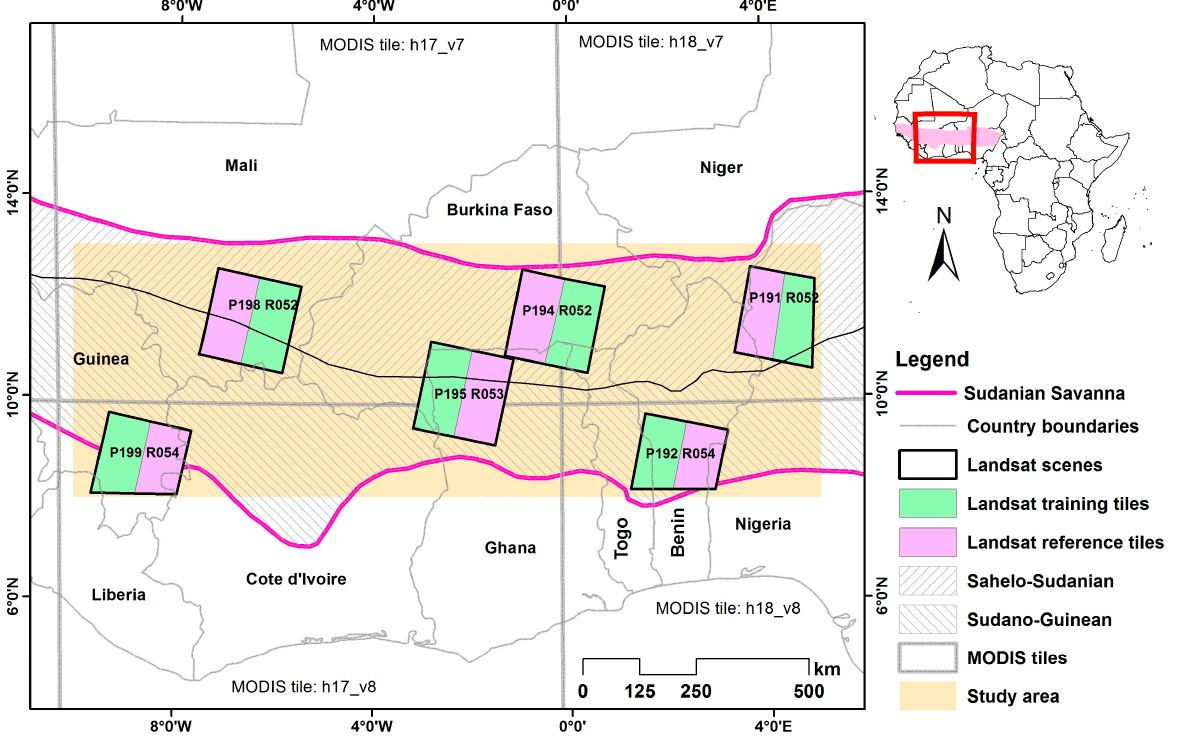
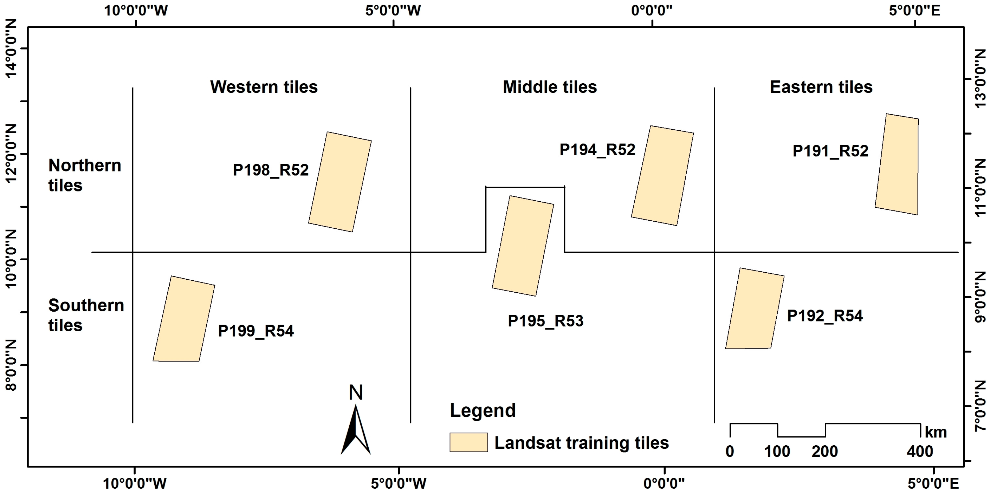
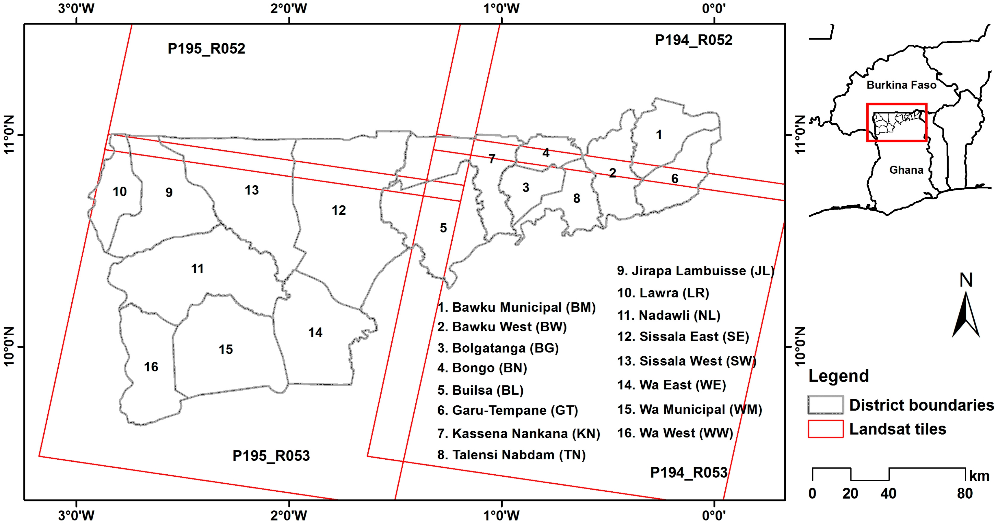
2.1. Study Area

The study was conducted in a 940,000 km2 area within the Sudanian Savanna agro-climatic region (Figure 1). The area covers parts of Mali, Guinea, Cote d’Ivore, Burkina Faso, Ghana, Togo, Benin, Niger and Nigeria. The agro-climatic zone is characterized by a mono-modal (single peak) rainfall distribution and high temperatures. Typically, rainfall lasts from May to October during which major agricultural activities are undertaken [31]. Total annual rainfall ranges between 500 and 1100 mm, although this is highly variable in space and time (inter and intra-annual) [32]. Average temperature in the zone ranges from 24 °C to 32 °C in the south and north, respectively [31]. The Sudanian Savanna zone is sometimes divided into a northern semi-arid region (Sahelo-Sudanian) with a mean annual rainfall range of 500 to 800 mm and a southern sub-humid region (Sudano-Guinean) having 800 to 1100 mm mean annual rainfall [32,33] (Figure 1). These two sub-divisions represent a climate gradient, with the Sudano-Guinean region having favorable climate conditions and a higher vegetation/tree cover. Consequently, tree crops (e.g., mangoes) and sub-canopy cultivation are more popular in the south than the north.
Agriculture is the predominant land use in the Sudanian Savanna zone. Rapid population growth and increasing land pressure have resulted in a change of the cropping system from shifting cultivation, a system in which a relatively long period of fallow follows a relatively short period of continuous cultivation [34] to intercropping, a system where farmers cultivate multiple crops on the same piece of land on a yearly basis [35,36]. Millet, maize, sorghum, rice, cotton and yam are the major crops cultivated. Dixon et al. [37] described the Sudanian Savanna as having the potential to become the breadbasket of West Africa.
Agriculture, however, largely remains at subsistence level with low degrees of mechanization and nutrient input [38,39]. Farm sizes are generally small and range between 0.5 and 2 ha [40,41]. Farmers tend to increase production through cropland expansion instead of intensification [1]. Low levels of nutrient input (e.g., fertilizers), poor management practices such as annual burning of vegetation, transportation of crop residue (e.g., groundnut, sorghum/millet stalks) to homesteads and continuous cultivation (without fallow) have led to a continuous decline in soil organic matter content and subsequently decline in soil fertility in most parts of the Sudanian Savanna [42].

2.2. Data and Pre-Processing

2.2.1. Landsat

Multi-temporal Landsat data from the Operational Land Imager (OLI) sensor were utilized in this study. Data for six Landsat scenes (Figure 1) were downloaded free-of-charge from the USGS's (United States Geological Surveys) EarthExplorer data platform. The atmospherically corrected “Landsat surface reflectance” product [43] was used. Table 1 details the scene numbers and acquisition dates. All images were acquired during or after harvest (October to December), which signifies the end of the rainy season and the beginning of the dry season. This choice is based on the findings of [17,44] who argued that the cropland mask can be optimally derived in the harvest season. Persistent cloud cover during the peak of the cropping season, which largely coincides with the rainy season, limits the acquisition of cloud-free images during this period.
Six spectral bands of the OLI data were analyzed: blue, green, red, near infrared (NIR) and the two shortwave infrared (SWIR) bands. In addition, three spectral indices, Normalized Difference Vegetation Index (NDVI), Soil Adjusted Vegetation Index (SAVI) and Simple Ratio (SR), were calculated for each image. Previous research have shown the usefulness of these indices [29,45,46].

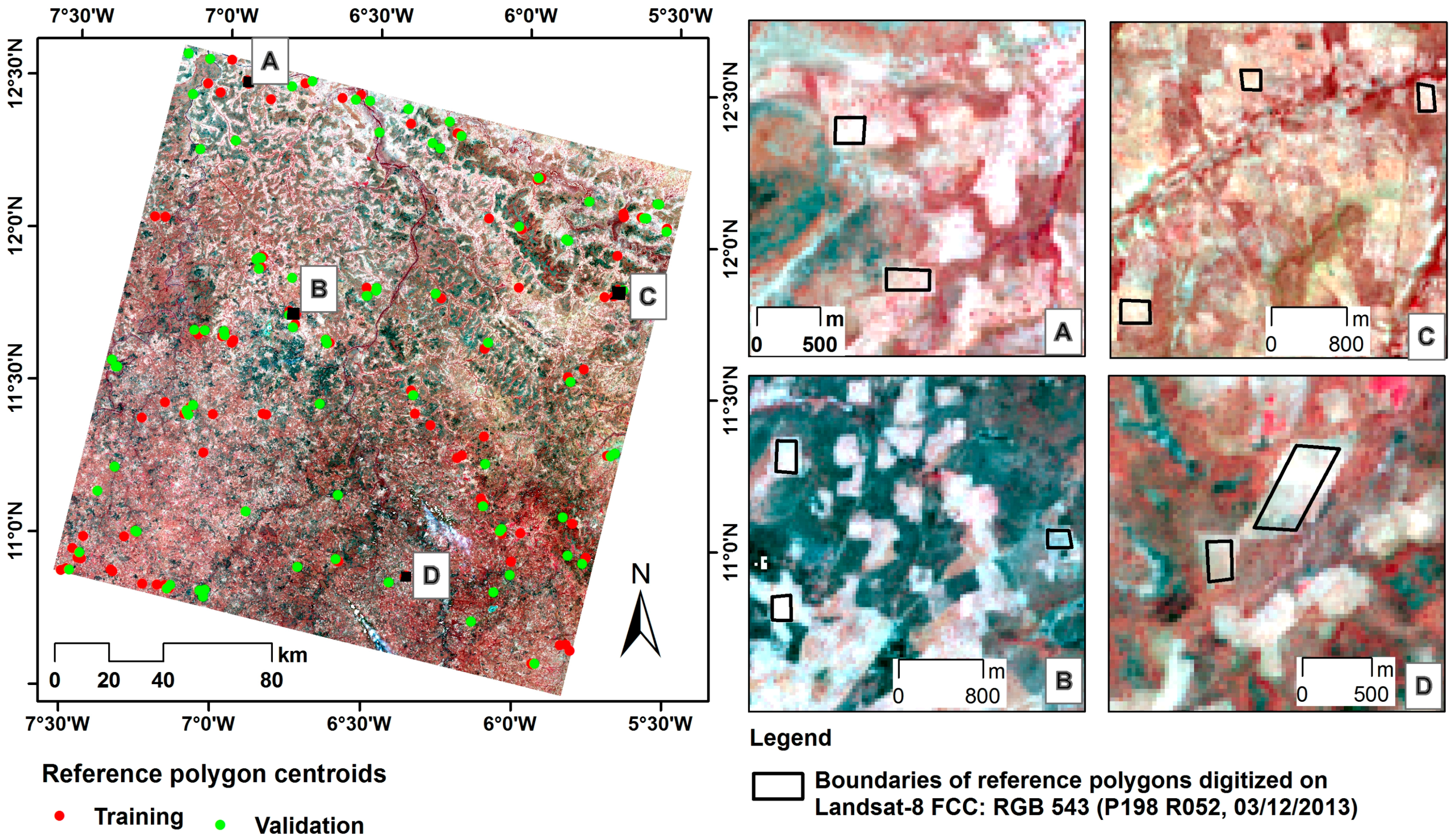
2.2.2. Reference Data

Reference data for classifying the Landsat images were digitized based on interpretation of image color composites augmented by Google Earth imagery. Reference data for four land use/land cover (LULC) classes—cropland, natural/semi-natural vegetation, artificial surfaces and water—were generated. Cropland in this context excluded fallow lands. Figure 2 shows a false color composite (FCC) of the Landsat scene P198_R052 (acquired on 3 December 2013) and detailed views of cropland reference polygons digitized on the FCC. In most cases, it was possible to delineate the LULC classes on the Landsat color composites with a high level of certainty. Pure pixels (i.e., without mixture of LULC classes) were selected as much as possible. However, due to the usage of harvest season images coupled with lack of clear cropland structure in certain areas, Google Earth images were sometimes used to generate reference data for such areas or to confirm a digitized polygon as truly representing cropland. All Google Earth images used were acquired on 31 December 2013. The digitized polygons were overlaid on the Landsat imagery and for each LULC class, a maximum of 2500 pixels were randomly selected as samples for training and validation. In some instances the maximum 2500 samples were not realized for some LULC classes due to the number and sizes of polygons digitized. Consequently, reference samples for each Landsat image ranged from 8000 to 10,000 pixels, and were divided (50% / 50%) into training and validation datasets for classification and accuracy assessment.

2.2.3. Moderate Resolution Imaging Spectroradiometer (MODIS)

Data from the standard MODIS product MOD13Q1 were downloaded free-of-charge from the MRTWeb interface [47] for the year 2013. This consists of twenty-three sixteen day composites, each composite comprising twelve layers. The layers of interest in this study were the three reflectance bands (red, NIR, and MIR), two vegetation indices (EVI and NDVI) and the reliability layer which provides a reliability rating for each pixel throughout the 16 day compositing period. The study region (Figure 1) falls within four MODIS tiles (h17v07; h17v08; h18v07; and h18v08). These tiles were mosaicked and subset with the online MRTWeb tool prior to downloading. The native resolution of 232 m was preserved, while the projection of the data was set to Universal Transverse Mercator.
Despite compositing daily acquisitions spanning sixteen days, persistent cloud cover during the cropping season (May–October) often lead to the MOD13Q1 product having low quality pixels. Therefore, the data were pre-processed using information in the reliability layer to produce a temporally consistent or smooth time-series by replacing invalid pixels (i.e., low quality pixels) through curve fitting [48]. The TIMESAT software was used [48]. The pre-processing entailed three steps. First, a suitable function was identified for each of the time-series (i.e., red, NIR, MIR, NDVI, EVI) using the “TSM_GUI” module of the software. Information contained in the pixel reliability layer was used as a quality indicator. A subjective weight of “1” was given to all pixels with reliability of “0”, “0.5” for pixels with reliability of “1 or 2” and “0” for pixels with reliability of “3”. Visual analysis revealed that an adaptive Savitzky–Golay filter with a window size of two [49] provided the best fit for all the time-series analyzed. The Savitzky–Golay filter operates with the moving window concept and replaces data values by a linear combination of nearby values in the window. In its operation, a quadratic polynomial is fitted to all points within a defined window by the method of linear least squares [49]. In the second step, the “TSF_Process” module of the software was used to fit the Savitzky–Golay function to the various time-series. Finally, the fitted/smoothed data were used to create a new set of images using the “TSF_fit2img” module of TIMESAT. TIMESAT seasonal metrics were not calculated.

2.2.4. MODIS Land Cover Product (MCD12Q1)

The MODIS Land Cover Product (MODIS_LCP) is a 500 m spatial resolution global map produced by the Boston University on an annual basis. The product is a result of a supervised (decision tree) classification of multi-spectral and multi-temporal MODIS data with an overall accuracy of approximately 75% [24]. It is provided in five global land cover classification systems including that of the International Geosphere-Biosphere Program (IGBP), which was extracted for this study.
The MODIS_LCP for the year 2013 was obtained free-of-charge from the USGS [50]. For purposes of this study, the two cropland classes in the product were extracted and used for qualitative and quantitative comparison. The two classes are defined as follows [51]:
  • Cropland (class 12): “Land cover with temporary crops followed by harvest and bare soil period (e.g., single and multiple cropping systems). Note that perennial woody crops will be classified as the appropriate forest or shrub land cover type”.
  • The Cropland/Natural Vegetation Mosaic (class 14): “Land with a mosaic of croplands, forest, shrublands, and grasslands in which no one component comprises more than 60% of the landscape”.

2.2.5. GlobeLand30

GlobeLand30 is a 30 m spatial resolution global LULC product derived from the classification of Landsat (TM and ETM+) and HJ-1 satellite images using a pixel-object-knowledge based (POK-based) approach [21]. Analyses were done for the baseline years 2000 and 2010. Validation of the product revealed an overall classification accuracy of over 80% [21]. Thus far, very few studies have validated the product over West Africa [13].
In this study, six GlobeLand30 tiles of the year 2010 that coincide with the Landsat tiles were obtained from [52]. To ensure comparison with the Landsat scale analysis, the ten LULC classes were reclassified into four classes. These are (GlobeLand30 classes are in parenthesis): (1) cropland (cultivated land); (2) natural/semi-natural vegetation (forest, grassland shrubland); (3) artificial surfaces (artificial surfaces, bare land); and (4) water (water bodies, wetlands). Two classes (tundra and permanent snow and ice) are not found in West Africa.

2.2.6. Agricultural Statistics Data
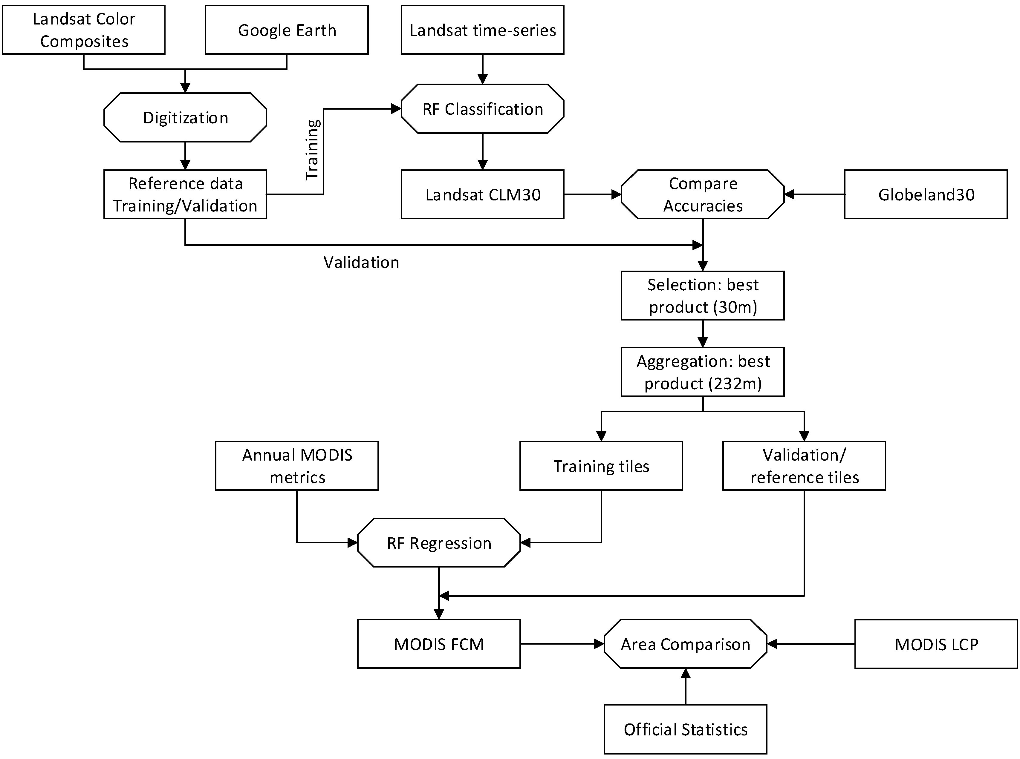
District level (2nd administrative level) agricultural statistics for Ghana were obtained from the Statistics, Research and Information Directorate (SRID) of Ghana’s Ministry of Food and Agriculture (MoFA) for the year 2013. The data consist of cropped area (ha), production (Mt) and yield (Mt/ha) of the major crops cultivated and are derived from surveys that are conducted by agricultural extension officers employed in each district. For this study, the total cropped area for sixteen districts was compared with remote sensing derived estimates in a plausibility analysis.

3. Methodology

Figure 3 summarizes the methodological approach. First, the 30 m multi-temporal Landsat images per scene (Table 1) were classified using the Random Forest classification algorithm to reveal four general LULC classes. Training data for the classification were derived from the generated reference data (from false color composites and Google Earth imagery—Section 2.2.2). Results of this analysis (Landsat_CLM30) were compared with the corresponding tiles from the GlobeLand30 by calculating accuracy statistics based on the validation set of the reference data (Section 2.2.2) and cropland area. It has to be noted that theoretically, the global coverage of GlobeLand30 makes it an ideal reference data for calculating fractional cropland cover at MODIS scale. However, the limited validation of this product over West Africa is a concern, hence the comparison. The Landsat scale product (Landsat CLM30 or GlobeLand30) which produced the best accuracy and cropped area estimates was selected to serve as the training/validation data for the calculation of fractional cropland cover at MODIS scale. The cropland class of the selected Landsat scale product was extracted and aggregated to the native resolution of MODIS (232 m). The aggregated Landsat scale data were divided into two halves: one for training (hereinafter referred to as “Landsat training tiles”), i.e., modeling the fractional crop cover and the other half for validating the results (hereinafter referred to as “Landsat reference tiles”) as shown in Figure 1.
The aggregated results of all the training tiles (six) were combined with corresponding values in the annual MODIS metrics to model fractional cropland cover using Random Forest regression. The developed model was applied to the annual MODIS metrics to predict fractional cropland cover for the entire study area.
Several experiments were conducted based on the hypothesis that generating a single model with all six training tiles could negatively affect the model’s predictive capacity due to the possibility of the tiles representing diverse factors such as soil types, vegetation dynamics (e.g., crop types, intercropping), or climate. Specifically, the experiments sought to: (1) determine whether using a subset (geographically) of the training data to generate a model can achieve results comparable to that when all tiles are used; and (2) determine how far the prediction power of a model can extend before significant reduction in accuracy can be observed. To achieve this, eleven experiments were conducted with each of the six tiles, pair of tiles (Western, Middle and Eastern) and three tile combinations (Northern and Southern) (Figure 4). In each experiment, a fractional cropland cover map was generated using a subset of the training data, i.e., single tile, pair of tiles or three tile combinations. All experiments followed the methodology explained in Section 3.2.
All generated fractional cover maps were validated using the aggregated results of the reference tiles. Finally, cropped area estimates derived from the fractional cover map were compared with corresponding estimates from the MODIS LCP and agricultural statistics to ascertain the level of agreement between them.

3.1. Landsat Classification

The multi-temporal Landsat images were classified into four broad LULC classes: (1) cropland; (2) natural/semi-natural vegetation (e.g., forest, grass, shrub and their mixture); (3) artificial surfaces (e.g., settlements, bare land, tarred roads, etc.); and (4) water bodies. The class of interest, however, was cropland. Cropland in this context refers to cultivated areas in the 2013 cropping season, excluding fallow lands.
The Random Forest (RF) package in the “R” statistical software was used to classify the images. RF [53] belongs to the family of ensemble machine learning algorithms that predicts a response (e.g., a class or fractional cover) from a set of predictors (matrix of training data) by creating multiple decision trees and aggregating their results. The training data (predictor/variable matrix) were derived by overlaying the digitized training polygons on the Landsat spectral bands and indices and extracting the underlying values. Based on this training matrix, RF generated 500 classification trees, with each tree built on a bootstrapped sample of the training data. At each node split, a sample of predictors, equivalent to the square root of the total number of predictors, were randomly selected as candidates for splitting. This approach reduces the correlation between trees and improves classification accuracy [53].

3.2. Calculation of Fractional Cover Maps

Random Forest Regression (RFR) was used to calculate fractional cropland cover at MODIS resolution using the Landsat classification results (Landsat CLM30) as training data. Compared to single regression trees, RFR has a higher predictive accuracy because it generates a large number of regression trees and combines the individual predictions through averaging [53]. Regression trees are constructed by recursively partitioning training data (from the root node) into disjointed regions (nodes) and providing a fitted value (cropland fractional cover in this case) within each region based on a set of predictors (independent variables). A response vector and a set of predictors are required for regression analysis. In this study, detected cropland areas at Landsat resolution which were aggregated to the same resolution as MODIS served as the response (dependent variable) while the MODIS annual metrics served as the predictors (independent variable). The aggregation was achieved by determining the proportion of Landsat cropland pixels within a MODIS pixel. After the aggregation, a stratified random sampling was performed to select pixels (5%) from the aggregated layer and their values (i.e., fractional crop cover) extracted to serve as the response vector in the RFR analysis. The predictor matrix was derived by extracting the corresponding values of the randomly sampled pixels from the MODIS time-series (i.e., red, NIR, MIR, EVI and NDVI). Based on the response and training data, the “randomForest” function in the RF package [54] was used to generate a regression model which was subsequently used to predict fractional cropland cover for the entire study area.
In generating the model, 200 regression trees (RTs) were constructed with a node size of 5. These parameters were selected after preliminary analysis was conducted using different parameters and noting the effect on accuracy [5]. The number of predictors randomly selected at each split (mtry) was set to the default of one-third of the total number of predictors [54].

3.3. Accuracy Assessment

Accuracy assessment was conducted at both Landsat and MODIS scales. At Landsat scale, the 50% validation dataset (see Section 2.2.2) was used to compute confusion matrices for the Landsat analysis and GlobeLand30. Overall, producer’s accuracy and user’s accuracy were noted. Additionally, the total cropland area under the respective reference tiles of both 30 m products were compared.
The aggregated results of the respective reference tiles (Figure 1) were used to assess the accuracy of the generated fractional cover map. Three model performance statistics were extracted (Equations (1)–(3)): (1) Mean Error (ME); (2) Mean Absolute Error (MAE); and (3) Root Mean Squared Error (RMSE). These statistics were computed for: (a) all pixels within each of the six reference tiles; and (b) combination of all pixels in all the six tiles.
M E = n 1 i = 1 n P i O i
M A E = n 1 i = 1 n | P i O i |
R M S E = n 1 i = 1 n ( P i O i ) 2 1 / 2
Next, the total cropland area calculated from the aggregated reference tiles (Figure 1) was compared with corresponding area estimates from the modeled fractional cover map and MODIS LCP. This was performed to assess the accuracy of the two products in estimating cropland area. In the case of the fractional cover map, cropland area was calculated based on Equation (4).
i = 1 n ( P i / 100 ) * P i x _ A r e a  
where P i is fractional cropland cover of the ith pixel; O i is the reference value for the ith pixel (i.e., aggregated classification results for the reference tile); n is the number of pixels in the spatial unit of analysis; and “Pix_Area” is the Area covered by a pixel.
In the case of the MODIS_LCP, cropland area was calculated from the two cropland classes as in Equation (5).
i = 1 N ( C i + ( D i * K ) ) * P i x _ A r e a
where C i represents class 12 of MODIS_LCP which can be considered as pure cropland (i.e., 100% cropland), D i represents cropland class 14 which is a mosaic of cropland and natural vegetation (see Section 2.2.3), “K” represents the proportion of D i that is cropland and “Pix_Area” is the area of a pixel. Estimating “K” is a challenge since according to the definition of class 14, it can range between 0% and 50%. However, for the purposes of comparison, a constant value of 0.5 (i.e., 50%) was used. This is in line with the assumptions made by previous studies (e.g., [3,10]).

3.4. Plausibility Analysis

A comparison was made between cropland area estimates from the remote sensing based LULC products and official cropped area estimates from Ghana’s Ministry of Food and Agriculture for sixteen administrative units (districts) in northern Ghana (Figure 5). Total cropland area within each district was determined from the fractional cover map (MODIS_FCM) and MODIS_LCP based on Equations (4) and (5). MoFA’s annual statistics include: (1) crop production (in metric tonnes); (2) cropped/harvested area (in hectares); and (3) yield (in metric tonnes per hectare) for all crops cultivated in each district. For purposes of this comparison, the total cropped area for each district was determined by summing the cropped/harvested area for all crops in the district.

4. Results

4.1. Classification Accuracy at Local Scale

The Landsat analysis (Landsat_CLM30) revealed more accurate results than GlobeLand30 (Table 2 and Figure 6) although the latter achieved an overall accuracy of more than 80% in four out of the six tiles. Nonetheless, the producer’s accuracy and user’s accuracy of the cropland class in GlobeLand30 were found to be very poor for three tiles (P199_54, P195_53, and P191_52), one of which recorded zero percent for both accuracy measures. In such instances, the overall accuracy of GlobeLand30 was mainly contributed by the other three non-cropland classes. On the other hand, the accuracy of the cropland class in Landsat_CLM30 consistently exceeded 90%, except that of P199_54. The use of harvest season images is a possible reason for the relatively high accuracy achieved for the Landsat_CLM30 results. This period affords the best separation between agricultural fields and surrounding natural vegetation due to a sharp reduction in, for example, vegetation indices on the former [5]. However, certain harvesting mechanisms of farmers in the Sudanian Savanna, where farmers transport crop residue to their homes for household usage [36,39], often lead to harvested fields being bare (Figure 7). Consequently, the main source of confusion for the cropland class (in Landsat_CLM30) was the artificial surfaces class.
The relatively low accuracies recorded for GlobeLand30, especially the cropland class, can be attributed to a number of factors. First, the reference data used for the validation of GlobeLand30 (produced with data of 2010) were generated from 2013 images. Thus, changes in cropland extent between 2010 and 2013, though not expected to be high, is a possible contributory factor to the low accuracies observed. Second, the integrated pixel, object and knowledge (POK) based approach adopted by Chen et al. [21] could have led to low accuracies in parts of the Sudanian Savanna where tree coverage is high and the landscape is very fragmented [5]. The application of object based approaches in such landscapes can easily lead to under or over detection of cropland due to high heterogeneity. Not surprisingly, worse accuracy estimates for GlobeLand30 were derived for tiles that are in the southern part of the study area, where tree cover and landscape fragmentation is high. Third, Chen et al. [21] admitted to confusion between cropland and bare areas/artificial surfaces, which could have been pronounced in West Africa due to the use of harvest season images vis-à-vis common harvesting approaches.
In addition, Figure 6 highlights that except for two tiles (P192_R54 and P194_R52), GlobeLand30 underestimated cropland area by about 50% or more. Consequently, Landsat_CLM30 was used in estimating fractional cropland cover at MODIS scale.

4.2. Accuracy Assessment at the Regional Scale

Table 3 presents the model performance statistics (ME, MAE, RMSE, and r-square (R2)) computed for the modeled fractional cropland cover. Aggregated classification results of the reference tiles served as the reference (true value) in the computation of the statistics. Statistics were computed separately for each of the six Landsat tiles as well as for all tiles combined. The number of validation samples considered in each case is presented in the table (“number of cells”).
Although the RMSE is an often used statistic to describe average model error, the MAE has been found to be a better statistic for model evaluation [55]. RMSE has a lower limit fixed at MAE, while its upper limit is the product of the square root of the number of samples and MAE (n1/2MAE) [55]. Thus, the MAE is used as key performance indicator in this study.
According to Table 3, a MAE of 19.1% was achieved for the fractional cropland cover (MODIS_FCM) when it was assessed with all the validation samples in the six reference tiles. However, validation using samples from the separate tiles revealed a variation in MAE from 21.3% (percent coverage) in the southeastern part of the study area (P192_R52) to 17.6% in the southwestern part (P199_R54). This together with a standard deviation of 1.37% (MAE) indicates a high level of consistency in accuracy over the study area. Apart from the MAE obtained for all reference samples, MODIS_FCM achieved good statistics at individual tile level. The variability in accuracy observed across the study area has been reported by other studies that assessed other global products. For example, in assessing the accuracy of an improved global LULC map, Leroux et al. [3] reported variability in accuracy across 55 validation sites where high resolution images were classified into crop and non-crop areas through photo interpretation. For West Africa, they found a considerable variation in accuracy of between 47% and 70%. Compared to their estimates, errors in the MODIS_FCM can be considered to be consistent due to the aforementioned relatively small variation in MAE, although the number of validation sites used could have influenced the degree of variation. In terms of overall accuracy, the value obtained in this study represents a significant improvement over the reported 51% for the MODIS_LCP [3], which has been found to have a better accuracy than most global LULC products [10].

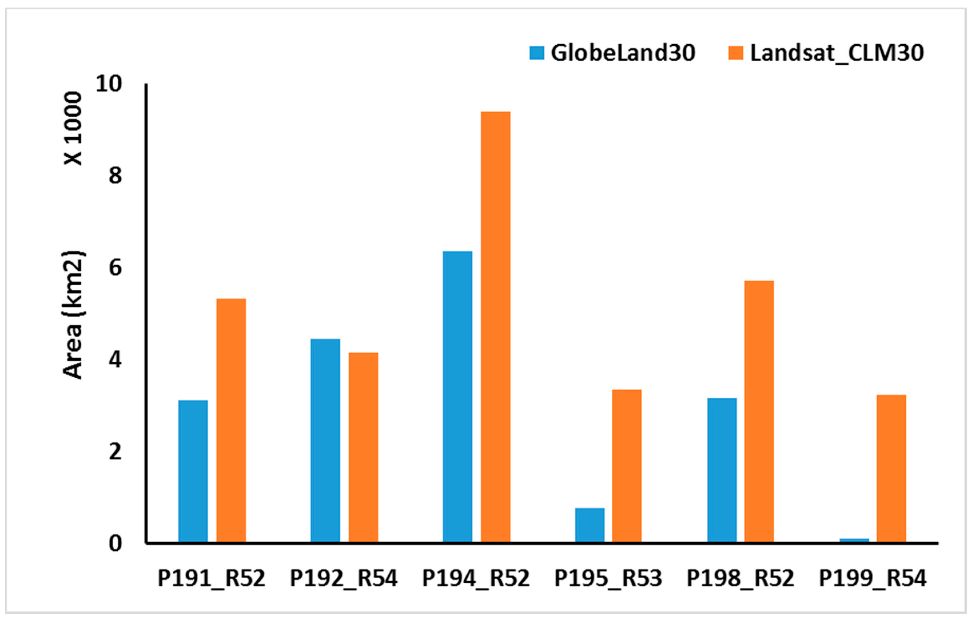
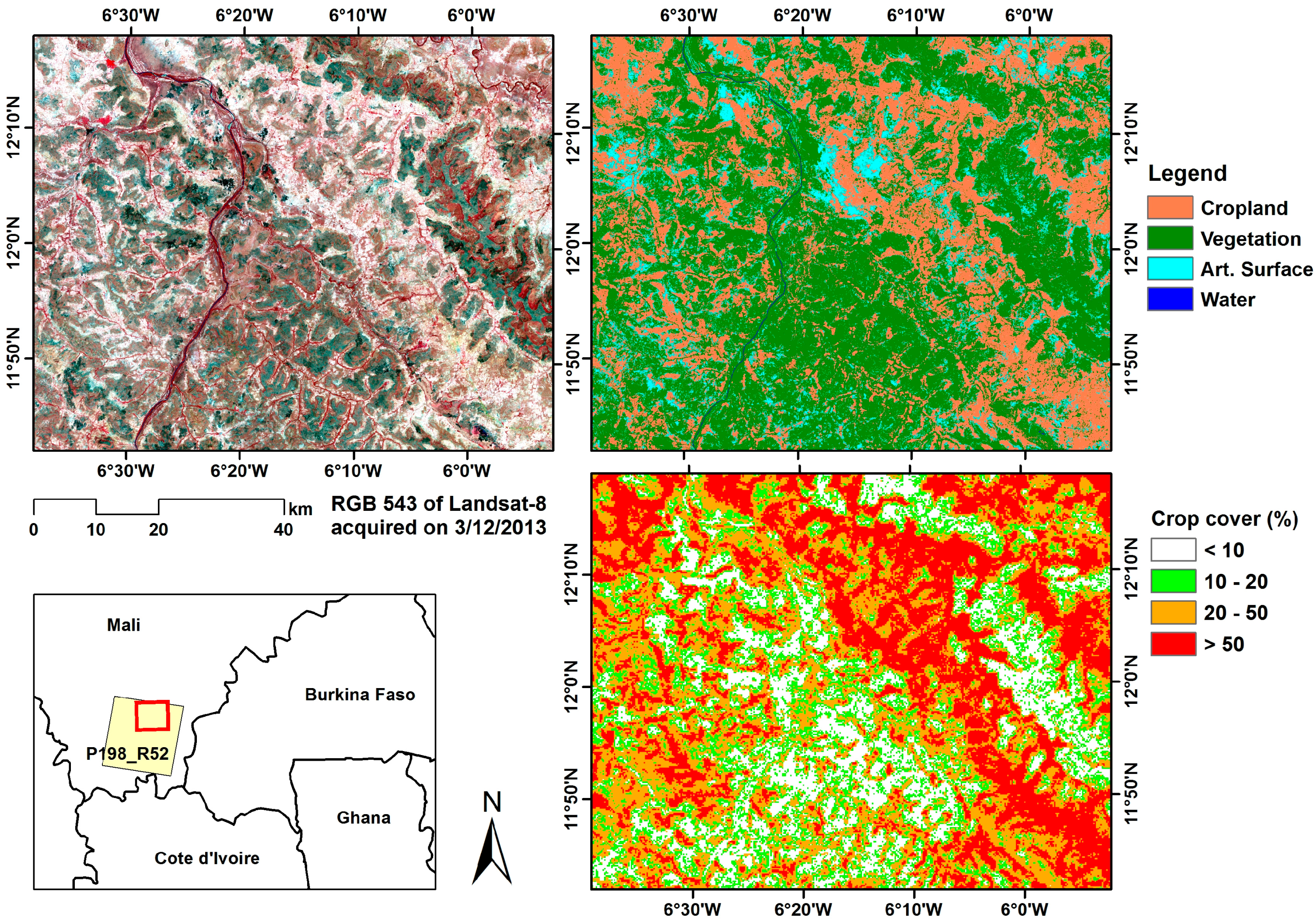
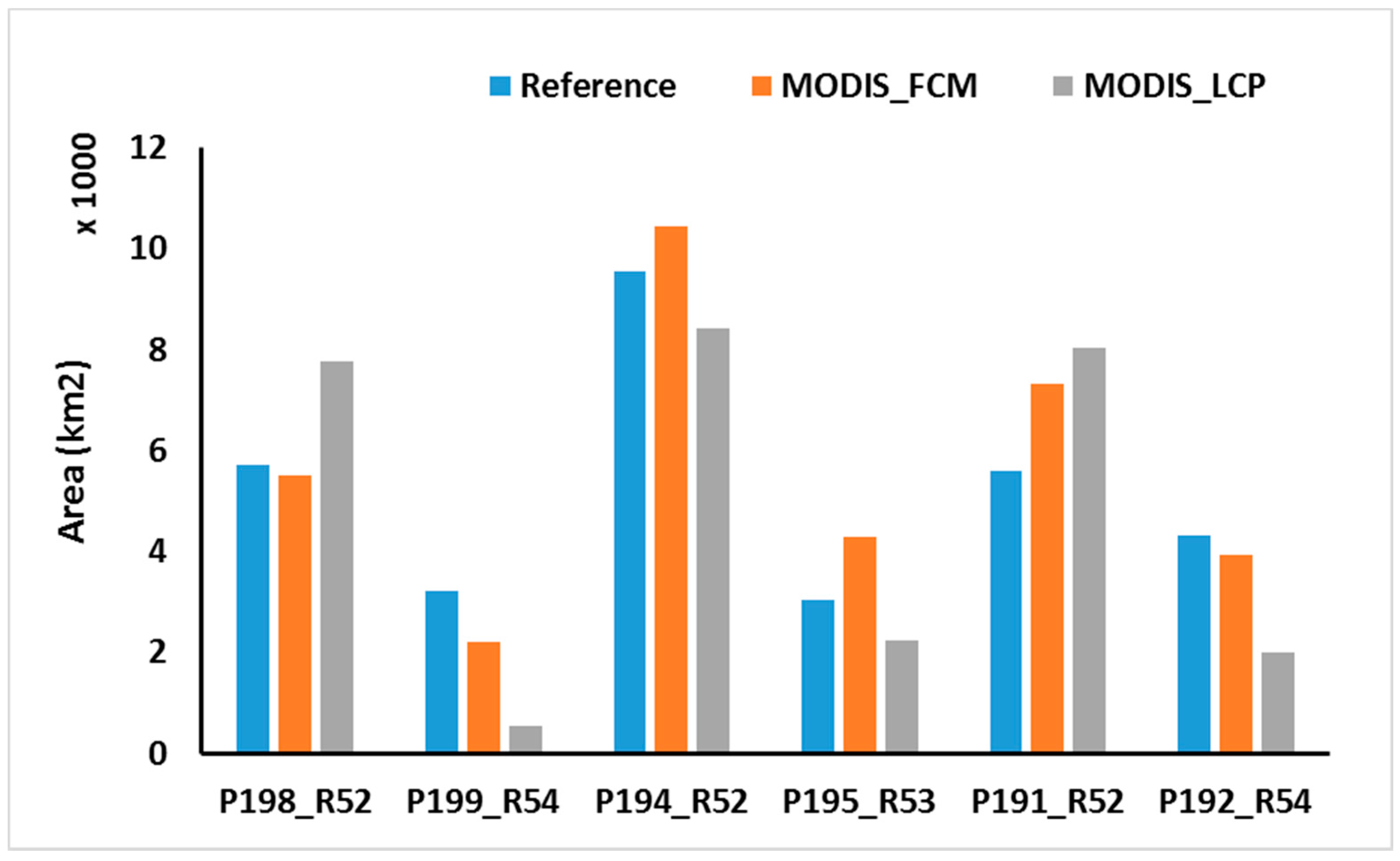
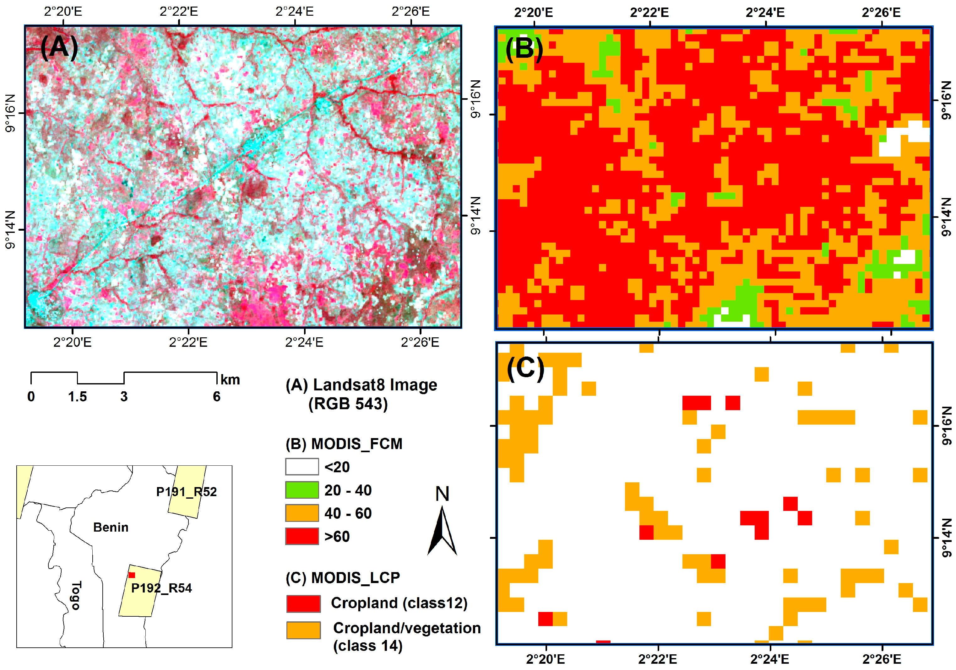
4.3. Spatial Distribution of Cropland and Area Assessments

The MODIS_FCM reasonably replicated the land cover pattern of the Landsat_CLM30 (Figure 8). Vegetated areas detected at Landsat scale were modeled as having either a fractional cropland cover of less than 10% (white areas) or between 10% and 20% (light green). The assignment of a cropland proportion to these areas can be explained by misclassifications between cropland and natural vegetation at the Landsat scale as well as by the problem of mixed pixels. The wrongful assignment of most vegetated areas as having crop cover of between 0% and 20% (Figure 8) is in line with the range and average of MAE at the validation stage (17.6%–21.3%) (Table 3). Consequently, areas with fractional cropland cover of between 0% and 20% are classified as one class in subsequent illustrations.
The northern part of the Sudanian Savanna region exhibited a generally high cropland share than the southern part (Figure 9a). Areas north of latitude 11.5° consistently have a fractional cropland cover of 60% (per MODIS pixel) or more. On the other hand, most of the areas south of latitude 11.5° have a cropland percentage (per MODIS pixel) of between 20% and 40%, while a few areas have a fractional cover of 60% or more. A visual inspection of Google Earth images confirmed the observed north–south gradient in cropland cover in the study area.
The MODIS_LCP for 2013 (Figure 9b) largely confirms the existence of the north–south gradient in cropland cover, with the northern parts having a greater percentage of cropland than the southern part. Nevertheless, a comparison of the MODIS_FCM with the MODIS_LCP is hampered because the first is derived from regression analysis and the second returned from a classification. Thus, croplands in pixels with a comparatively low cropland percentage for instance in the southern part of the study area remain undetected when using the classification approach.
Cropland area summarized for the six Landsat reference tiles extracted from: (1) the reference (i.e., aggregated Landsat_CLM30); (2) MODIS_FCM; and (3) MODIS_LCP is given in Figure 10. The MODIS_FCM generally overestimated cropland in the northern part of the study area and underestimated cropland in the southern part when compared to the reference. Out of the three northern reference tiles (see Figure 4), MODIS_FCM overestimated cropland in two tiles by 9% (P194_R52) and 31% (P191_R52) and underestimated cropland by 4% for P198_R52. On the other hand, MODIS_FCM underestimated cropland for two out of the three southern tiles by 9% (P192_R52) and 32% (P199_R54) and overestimated cropland by 41% for P193_R53. These are in line with the mean error (ME) estimates in Table 3. Positive ME indicates that the MODIS_FCM is positively biased and therefore overestimate cropland while negatively biased areas (negative ME) underestimates cropland. The overall ME of +2.267, however, shows that the MODIS_FCM generally overestimate cropland which averages at about 6%. The MODIS_LCP also overemphasized cropland in the northern part of the study area for two tiles by 35% (P198_R52) and 43% (P191_R52) and underestimated cropland for all other tiles by 83% (P199_R54), 26% (P195_R53), 53% (P192_R54) and 11.8% (P194_R52), resulting in a net underestimation of 16%.
Compared to the reference, the MODIS_FCM performed better than MODIS_LCP in terms of cropped area estimation. Based on calculated cropland percentages in the reference tiles, the MODIS_FCM achieved a MAE of 5.57% against 12.4% for MODIS_LCP. This translates into an accuracy of 94% and 88% for the MODIS_FCM and MODIS_LCP, respectively (i.e., at the scale of the reference tiles). These statistics suggest that determining the fractional proportions of cropland on coarse spatial resolution images such as MODIS may be a better way of providing cropped area estimates in heterogeneous and fragmented landscapes (Figure 11).

4.4. Impact of Training Samples on Regional Cropland Mapping

Results of the experiments conducted to assess the impact of the quantity and spatial distribution of training samples on model accuracy are presented in Table 4 and Table 5. Table 4 presents results when single tiles were iteratively used as training data to predict fractional cropland cover while Table 5 show results obtained when a combination of tiles were used for model prediction (see Figure 4). Each model result was validated with the individual reference tiles (e.g., P198_R52) as well as all reference tiles together (“All”) and the MAE in each case calculated. The values in the tables represent the difference between the MAE achieved when all six tiles were used for model prediction and when single or a combination of tiles were used for prediction. Thus, negative values indicate instances where the experiment returned a higher error (MAE) compared to the error achieved when all six tiles were used for model prediction (see Table 3). Accordingly, positive values indicate a reduced error. Subscript numbers in Table 4 represent the straight-line distance between each of the single training tiles used for model prediction and the other five tiles. Here, distances were measured from the centroids of the training tiles.
Table 4 indicates that prediction with the single tiles led to an improvement in MAE (1.2%–4.4%) when validated with the respective adjoining reference tiles (leading diagonal in Table 4). This suggest that the predictive power of the respective models were sufficient to accurately predict fractional cropland cover within a distance of zero to about ninety kilometers (half width of Landsat tile) east or west of the training data. Proximity of the training and reference tiles, and the possibility of the adjoining areas having similar biophysical properties or belonging to the same “local” agro-ecological zone is a possible reason for this observation [56].
However, the results (off-diagonal in Table 4) do not show a clear pattern with respect to distance, i.e., model’s predictive power does not necessarily reduce or increase with distance, although in most cases worse MAE statistic was obtained (negative values). Whereas in some few cases an improvement in MAE was recorded for reference tiles that are relatively close to the training tile, worse MAE was recorded for most reference tiles whether relatively close to, or far from, the training tile. For example, the model generated with tile P198_52 recorded an increase in MAE of 4.8% when validated with reference tile P195_53 which is about 407 km away but recorded a decrease of 5.1% when validated with reference tile P199_R54 which is also just about the same distance from the training tile (437 km). On the other hand, an improvement of 3.3% was recorded when the model generated with P192_R54 was validated with the reference tile P199_R54 which is 1197 km away but a reduction in MAE of 18.4% was observed for reference tile P194_R52 which is just 342 km away. This may be indicative of the complexity of the landscape in the Sudanian Savanna zone and a possible non-linear relationship between factors that influence cropland area in one part of the zone and another. In addition, variation in image acquisition dates (Table 1) may be one reason for the deviations.
This notwithstanding, using tiles in the northern part of the study area generally produced relatively low MAE estimates compared to southern tiles. Prediction with the northern tiles (P198_R52; P194_R52; and P191_R52) produced lower overall MAE (column “All”) than the southern tiles (Table 5). In addition, the overall prediction error obtained when all three northern tiles were used together (Table 5) is almost identical to that achieved when all six tiles were used for prediction (0.6% difference). Compared to the northern tiles, the model generated with only southern tiles performed very poorly when validated against northern reference tiles (Table 5), recording a high average prediction error compared to when all six tiles were used (9.6% difference). These differences between northern and southern tiles can be linked to the two sub-climatic zones in the Sudanian Savanna, i.e., the northern semi-arid Sahelo-Sudanian zone and the southern sub-humid Sudano-Guinean zone (Figure 1). The prevalence of sub-canopy cultivation and high tree cover (tree plantations) in the southern sub-humid zone is a possible cause of the relatively poor performance of the southern tiles. The results indicate that in the event of limited resources (financial, data, human, etc.), it may be better to focus/purchase satellite images in the northern part of the study area to be used as training samples for regional scale cropland mapping/monitoring.
However, although the overall prediction error was minimal when the three northern tiles were used for model generation, significant errors were recorded for some southern reference tiles (i.e., P199_R54 and P192_R54). The inclusion of the southern tiles (i.e., the use of all six tiles) produced optimal results in terms of overall and tile specific prediction error. This suggests that when resources are available, or freely available imagery is being used as in this case, as many tiles as possible are needed to achieve optimal results. This will reduce the effect of the landscape fragmentation and the effect of diverse agro-ecological zones on the predicted fractional cropland and produce reasonable results for regional scale mapping. The results in Table 4 and Table 5, therefore, suggest to reject the hypothesis that model generation with samples from areas of potentially different climate, soil, vegetation, etc. can negatively affect the predictive accuracy of the model within the study area.

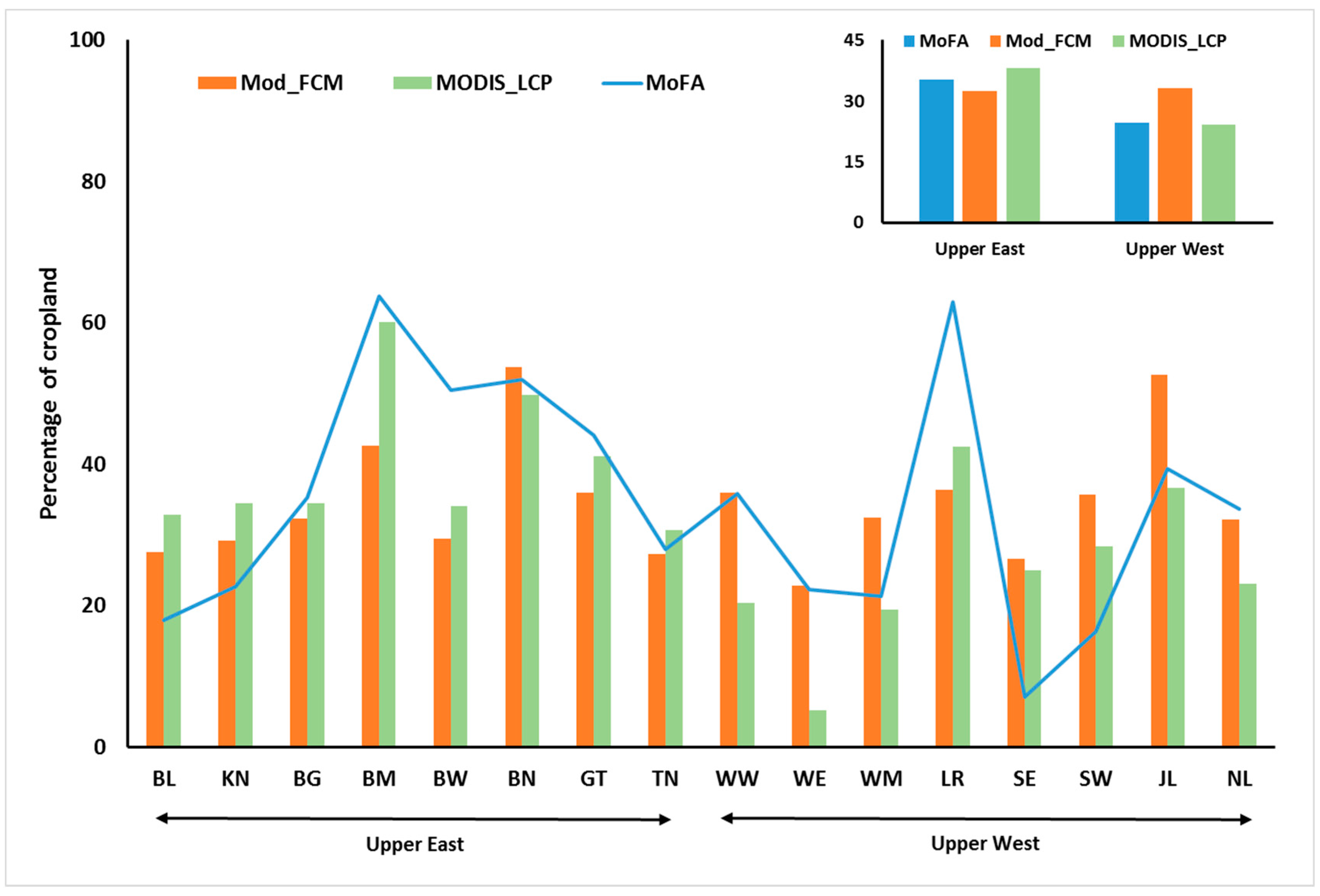
4.5. Plausibility Analysis Using Official Census Data

Variable levels of agreement and partly enormous disagreements between cropped area estimates from official government statistics (MoFA), MODIS_FCM and MODIS_LCP were found for sixteen districts in the Upper East (UER) and Upper West (UWR) regions of Ghana (3% of the study area). Given MoFA estimates as a benchmark, MODIS_FCM and MODIS_LCP recorded a net overestimation of 18.1% and 2.1%. Even higher variability among the datasets becomes visible at the district level (Figure 12). These deviations in cropped area at different scales, even among the remote sensing products, confirm observations made by previous researchers about the generally low level of agreement in such comparisons [11,12]. On the other hand, the graph shows a relatively increased congruence between the three data sources for districts in the UER (standard deviations of 15.9, 9.2, and 10.3 for MoFA, MODIS_FCM, and MODIS_LCP respectively) than those in the UWR (standard deviations of 17.2, 8.8, and 11.3 for MoFA, MODIS_FCM, and MODIS_LCP, respectively.

5. Discussion

Results obtained in this study demonstrate the potential of fractional cover approaches to improve the representation of cropland in heterogeneous landscapes. The range of MAE values achieved for MODIS_FCM compare favorably with other studies that used regression-based approaches to estimate the fractional proportions of other land cover types. For example, Tottrup et al. [57] used regression tree modeling and MODIS data to model the fractional cover of mature forest, secondary forest and non-forest and reported MAE of 14.6%, 21.6% and 17.1%, respectively. Although low R2s were achieved for some validation tiles (Table 3), the average R2 of 0.51 is comparable with other studies that evaluated fractional crop cover based on R2. Verbeiren et al. [58], for instance, modeled crop area fractions of two major crops in Belgium (winter wheat and maize) using artificial neural networks and conducted a pixel based comparison with actual crop area derived from a national land use map and reported an R2 of 0.58 and 0.54 for winter wheat and maize, respectively.
The range of RMSE obtained for MODIS_FCM (22.9 to 26.5) is remarkably lower than what was reported in Gessner et al. [29]. Gessner et al. [29] reported RMSEs of between 3.1% and 9.9% for the estimation of fractional cover of natural vegetation and bare surfaces in Namibia. However, they used very high resolution images (Quickbird and IKONOS) to map natural vegetation and bare surfaces before upscaling the results unto Landsat and MODIS resolutions. The use of very high resolution images can enable a better detection of land cover units and subsequently the derivation of more realistic cover proportions to be used as training data (response) in the regression analysis. In this regard, the spatial resolution limitations of Landsat vis-à-vis the heterogeneous landscape in the Sudanian Savanna region is believed to be the primary source of error in MODIS_FCM derived in this study. Due to the fact that a per-pixel classification approach was adopted at the Landsat scale, a pixel classified as cropland could have a portion of it as natural vegetation [59]. This is particularly the case in the southern part of the Sudanian Savanna region, where the prevalence of sub-canopy cultivation results in many trees on agricultural plots (agroforestry systems) [60].
MODIS_FCM showed a north–south gradient in cropland distribution, with the north having a higher cropland percentage than the south (Figure 9). Compared to the south, heavy reliance of the population in the northern part of the study area (i.e., north of latitude 11.5°) is one reason for this disparity. Sanfo [61], for example, reported that more than 86% of the population in Burkina Faso are employed by the agricultural sector, while the figure is between 50% and 60% for Ghana [62,63]. This could lead to cultivation of extensive areas in Burkina Faso (which forms part of northern Sudanian Savanna) than Ghana which is in the south. The occurrence of relatively poor soils and low rainfall distribution in the northern part compared to the south is another possible explanation. Whereas some studies stated that declining soil fertility can lead to farmers abandoning their lands [64,65], others reported that declining soil fertility, which results in low yields, cause farmers to expand production into marginal lands as a survival strategy and insurance against low yields [1,66,67]. This normally happens in areas of land scarcity, where the traditional fallowing system of abandoning land for a period can no longer be supported [66]. In addition, declining rainfall and a drier climate have been found to be an incentive for some farmers, especially those in the Sudano-Sahelian region, to expand cultivated area as an insurance against poor yields or crop failure [1,68,69]. The prevalence of bare soils in the northern part, and the observed misclassification between cropland and bare soils at Landsat scale, is believed to be one of the reasons for the general overestimation of cropland by MODIS_FCM and MODIS_LCP in that part of the study area (see Section 4.3).
However, although the northern part may genuinely have a higher cropland proportion, high occurrence of vegetation (especially trees), tree plantations (e.g., mangoes), and the predominance of agroforestry (cultivation under trees) in the southern part are believed to have contributed to the low proportion of croplands detected. In the south, relatively favorable climatic and environmental conditions occur [1]. Thus, spectral similarities between such plantations and ordinary trees (e.g., on croplands) can result in confusion between natural vegetation and cropland and tree-covered croplands may have remained undetected even in the Landsat classification and consequently in the MODIS based regression. This situation could have contributed to the general underestimation of cropland by the two MODIS products, although that of MODIS_LCP was quite pronounced. The low spatial resolution of MODIS_LCP and the per-pixel approach limits its usefulness for estimating cropland area. Previous studies (e.g., [3]) have noted that the assumption of 100% and 50% cropland for classes 12 and 14 respectively of MODIS_LCP is problematic because in actual fact, cropland proportion in class 12 may vary between 60% and 100% while class 14 could be between 0% and 50%. This suggests that using the highest possible cropland proportion in each class should yield the highest possible cropland area for each of the reference tiles. However, the magnitude of, for example, cropland underestimations in the southern part of the study area (i.e., 26%–83%) by MODIS_LCP indicates possible significant flaws in the product with regards to cropland area estimation.
Comparison of crop area estimates from the MODIS products with official agricultural census data revealed varying degrees of agreement and disagreements between the two sources. Nevertheless, there is a strong possibility of having errors in official government statistics (e.g., [59,70]). Ramankutty [71] explained that such errors in official crop area statistics could be due to either: (1) a deliberate under- or overestimation due to certain incentives (e.g., reducing tax burdens and artificially inflating crop productivity figures [72]); or (2) the lack of resources or adequate infrastructure to conduct rigorous and reliable surveys. Belshaw [73], for instance, observed that cropped area in Uganda was underestimated in 1965 due to farmers' non-disclosure of the location of all their distant plots for fear of increased tax. In Ghana, lack of resources (human and financial) and inadequate infrastructure (e.g., road access) is believed to be the main cause of the possible errors in the MoFA statistics for certain districts. During agricultural census, MoFA divides a district into enumeration areas (EAs), from which a sample is selected to be surveyed. Within each selected EA, a sample of farms are further selected and surveyed by trained agricultural extension officers. Since each district conducts its own survey with limited coordination, different estimation accuracies could be obtained depending on: (1) size of the district vis-a-vis the number of EAs selected (i.e., statistical significance of the sample); (2) availability of adequate road access to enable enumerators reach all sampled EAs; (3) level of training and experience of enumerators; and (4) availability of adequate and accurately/regularly calibrated tools (e.g., compasses, measuring tapes, GPS handsets, etc.). Additionally, most enumerators, per FAO recommendation [71], subjectively estimate the area proportion of crops on an intercropped field, which could introduce further errors. Thus, differences in the financial, logistical, infrastructural and human resource base of the different districts could influence the quality of the estimations.

6. Conclusions

In this study, multi-temporal Landsat and MODIS data were integrated to map fractional cropland cover at MODIS resolution in the Sudanian savanna agro-ecological zone of West Africa using regression-based approaches. A comparison of cropland areas mapped from Landsat data (Landsat_CLM30) with a global Landsat scale LULC map (GlobeLand30) underline the need for more local scale validation of global LULC products, especially in smallholder dominated fragmented landscapes such as West Africa, and indicate the necessity of producing accurate local cropland maps for cropland cover fraction estimation at the MODIS scale.
Overall mean absolute error of the fractional cover map (MODIS_FCM) (19.1%) compares favorably with other studies that used regression-based approaches to estimate the fractional proportions of other land cover types. MODIS_FCM, however, assigned cropland proportions of between 0% and 20% to some purely vegetated areas, which could be partly traced to spatial resolution limitations of Landsat (30 m) and challenges in separating croplands from natural vegetation and bare soil. Latest sensor systems with improved spatial (10–20 m) and temporal resolution such as Sentinel-2 could overcome this challenge for heterogeneous landscapes as occur in West Africa and generate better cropland representations at local scale prior to upscaling to a moderate resolution imagery (e.g., MODIS or Sentinel-3).
At least for the study area and scale investigated, systematic selection of reference data from areas of diverse climate, soil type and vegetation dynamics does not negatively affect a model’s predictive capacity. Only the selection of reference data from the northern part of the Sudanian Savanna generally produced better results than data from the southern part.
Comparison of cropped area estimates from MODIS_FCM and the MODIS land cover product (MODIS_LCP) suggest that the fractional cover approach is better suited for realistic cropped area estimates in fragmented landscapes. Partly enormous disagreements between crop area estimates of MODIS_FCM and official government statistics show the need to integrate remote sensing approaches and ground based surveys in improving cropped area estimation especially for large and deprived areas with limited logistical and human resources.
The increased availability of open source remote sensing data (e.g., Sentinels, Landsat, MODIS, PROBA-V, etc.), in combination with the proposed approach, is expected to improve our knowledge of the spatial extent and temporal dynamics of cropland at varying scales. Operationalization of the proposed approach based on open source data can aid in assessing past and future trends in cropland area and subsequently lead to improved land and agricultural management.

Acknowledgments

Authors acknowledge financial support from the German Federal Ministry of Education and Research (BMBF) through the research project: West African Science Service Center on Climate Change and Adapted Land Use (WASCAL) (01LG1001A).

Author Contributions

Gerald Forkuor designed the study and conducted image analysis with guidance from Christopher Conrad. A first draft of the manuscript was written by Gerald Forkuor, which received substantial review from Christopher Conrad. All other authors contributed to improving the manuscript by providing valuable inputs.

Conflicts of Interest

Authors declare no conflict of interest.

References

  1. Ruelland, D.; Levavasseur, F.; Tribotté, A. Patterns and dynamics of land-cover changes since the 1960s over three experimental areas in Mali. Int. J. Appl. Earth Obs. Geoinf. 2010, 12, S11–S17. [Google Scholar] [CrossRef]
  2. Tilman, D.; Cassman, K.G.; Matson, P.A.; Naylor, R.; Polasky, S. Agricultural sustainability and intensive production practices. Nature 2002, 418, 617. [Google Scholar] [CrossRef] [PubMed]
  3. Leroux, L.; Jolivot, A.; Bégué, A.; Seen, D. Lo; Zoungrana, B. How Reliable is the {MODIS} Land Cover Product for Crop Mapping {Sub-Saharan} Agricultural Landscapes? Remote Sens. 2014, 6, 8541–8564. [Google Scholar] [CrossRef] [Green Version]
  4. Vancutsem, C.; Marinho, E.; Kayitakire, F.; See, L.; Fritz, S. Harmonizing and Combining Existing Land Cover/Land Use Datasets for Cropland Area Monitoring at the African Continental Scale. Remote Sens. 2013, 5, 19–41. [Google Scholar] [CrossRef] [Green Version]
  5. Forkuor, G. Agricultural Land Use Mapping in West Africa Using Multi-sensor Satellite Imagery. Ph.D. Thesis, University of Würzburg, Würzburg, Germany, 2014. Available online: http://opus.bibliothek.uni-wuerzburg.de/frontdoor/index/index/docId/10868 (accessed on 20 February 2015).
  6. Thenkabail, P.S.; Hanjra, M.A.; Dheeravath, V.; Gumma, M. A Holistic View of Global Croplands and Their Water Use for Ensuring Global Food Security in the 21st Century through Advanced Remote Sensing and Non-remote Sensing Approaches. Remote Sens. 2010, 2, 211–261. [Google Scholar] [CrossRef] [Green Version]
  7. Forkuor, G.; Cofie, O. Dynamics of land-use and land-cover change in Freetown, Sierra Leone and its effects on urban and peri-urban agriculture—A remote sensing approach. Int. J. Remote Sens. 2011, 32, 1017–1037. [Google Scholar] [CrossRef]
  8. Andrew Wardell, A.D.; Reenberg, A.; Tøttrup, C. Historical footprints in contemporary land use systems: forest cover changes in savannah woodlands in the Sudano-Sahelian zone. Glob. Environ. Chang. 2003, 13, 235–254. [Google Scholar] [CrossRef]
  9. Herold, M.; Mayaux, P.; Woodcock, C.E.; Baccini, A.; Schmullius, C. Some challenges in global land cover mapping: An assessment of agreement and accuracy in existing 1 km datasets. Remote Sens. Environ. 2008, 112, 2538–2556. [Google Scholar] [CrossRef]
  10. Vintrou, E.; Desbrosse, A.; Bégué, A.; Traoré, S.; Baron, C.; Lo Seen, D. Crop area mapping in West Africa using landscape stratification of MODIS time series and comparison with existing global land products. Int. J. Appl. Earth Obs. Geoinf. 2012, 14, 83–93. [Google Scholar] [CrossRef]
  11. Fritz, S.; See, L.; Rembold, F. Comparison of global and regional land cover maps with statistical information for the agricultural domain in Africa. Int. J. Remote Sens. 2010, 31, 2237–2256. [Google Scholar] [CrossRef]
  12. Hannerz, F.; Lotsch, A. Assessment of remotely sensed and statistical inventories of African agricultural fields. Int. J. Remote Sens. 2008, 29, 3787–3804. [Google Scholar] [CrossRef]
  13. Lambert, M.; Waldner, F.; Defourny, P. Cropland Mapping over Sahelian and Sudanian Agrosystems : A Knowledge-Based Approach Using PROBA-V Time Series at 100-m. Remote Sens. 2016, 8, 232. [Google Scholar] [CrossRef]
  14. Eberenz, J.; Verbesselt, J.; Herold, M.; Tsendbazar, N.E.; Sabatino, G.; Rivolta, G. Evaluating the potential of proba-v satellite image time series for improving LC classification in semi-arid African landscapes. Remote Sens. 2016. [Google Scholar] [CrossRef]
  15. Cord, A.; Conrad, C.; Schmidt, M.; Dech, S. Standardized FAO-LCCS land cover mapping in heterogeneous tree savannas of West Africa. J. Arid Environ. 2010, 74, 1083–1091. [Google Scholar] [CrossRef]
  16. Delrue, J.; Bydekerke, L.; Eerens, H.; Gilliams, S.; Piccard, I.; Swinnen, E. Crop mapping in countries with small-scale farming: A case study for West Shewa, Ethiopia. Int. J. Remote Sens. 2013, 34, 2566–2582. [Google Scholar] [CrossRef]
  17. Forkuor, G.; Conrad, C.; Thiel, M.; Ullmann, T.; Zoungrana, E. Integration of optical and synthetic aperture radar imagery for improving crop mapping in Northwestern Benin, West Africa. Remote Sens. 2014, 6, 6472–6499. [Google Scholar] [CrossRef] [Green Version]
  18. Lobell, D.B.; Asner, G.P. Cropland distributions from temporal unmixing of MODIS data. Remote Sens. Environ. 2004, 93, 412–422. [Google Scholar] [CrossRef]
  19. Ozdogan, M. The spatial distribution of crop types from MODIS data: Temporal unmixing using Independent Component Analysis. Remote Sens. Environ. 2010, 114, 1190–1204. [Google Scholar] [CrossRef]
  20. Olofsson, P.; Stehman, S.V.; Woodcock, C.E.; Sulla-Menashe, D.; Sibley, A.M.; Newell, J.D.; Friedl, M.A.; Herold, M. A global land-cover validation data set, part I: fundamental design principles. Int. J. Remote Sens. 2012, 33, 5768–5788. [Google Scholar] [CrossRef]
  21. Chen, J.; Chen, J.; Liao, A.; Cao, X.; Chen, L.; Chen, X.; He, C.; Han, G.; Peng, S.; Lu, M.; Zhang, W.; Tong, X.; Mills, J. Global land cover mapping at 30m resolution: A POK-based operational approach. ISPRS J. Photogramm. Remote Sens. 2015, 103, 7–27. [Google Scholar] [CrossRef]
  22. Loveland, T.R.; Belward, A.S. The IGBP-DIS global 1km land cover data set, DISCover: First results. Int. J. Remote Sens. 1997, 18, 3289–3295. [Google Scholar] [CrossRef]
  23. Mayaux, P.; Bartholomé, E.; Fritz, S.; Belward, A. A new land-cover map of Africa for the year 2000. J. Biogeogr. 2004, 31, 861–877. [Google Scholar] [CrossRef]
  24. Friedl, M.A.; Sulla-Menashe, D.; Tan, B.; Schneider, A.; Ramankutty, N.; Sibley, A.; Huang, X. MODIS Collection 5 global land cover: Algorithm refinements and characterization of new datasets. Remote Sens. Environ. 2010, 114, 168–182. [Google Scholar] [CrossRef]
  25. Thenkabail, P.S.; Biradar, C.M.; Noojipady, P.; Cai, X.; Dheeravath, V.; Li, Y.; Velpuri, M.; Gumma, M.; Pandey, S. Sub-pixel Area Calculation Methods for Estimating Irrigated Areas. Sensors 2007, 7, 2519–2538. [Google Scholar] [CrossRef] [Green Version]
  26. Zurita-Milla, R.; Gomez-Chova, L.; Guanter, L.; Clevers, J.G.P.W.; Camps-Valls, G. Multitemporal Unmixing of Medium-Spatial-Resolution Satellite Images: A Case Study Using MERIS Images for Land-Cover Mapping. IEEE Trans. Geosci. Remote Sens. 2011, 49, 4308–4317. [Google Scholar] [CrossRef]
  27. Amorós-López, J.; Gómez-Chova, L.; Alonso, L.; Guanter, L.; Zurita-Milla, R.; Moreno, J.; Camps-Valls, G. Multitemporal fusion of Landsat/TM and ENVISAT/MERIS for crop monitoring. Int. J. Appl. Earth Obs. Geoinf. 2013, 23, 132–141. [Google Scholar] [CrossRef]
  28. Zhu, C.; Lu, D.; Victoria, D.; Dutra, L.V. Mapping fractional cropland distribution in Mato Grosso, Brazil using time series MODIS enhanced vegetation index and Landsat Thematic Mapper data. Remote Sens. 2016. [Google Scholar] [CrossRef]
  29. Gessner, U.; Machwitz, M.; Conrad, C.; Dech, S. Estimating the fractional cover of growth forms and bare surface in savannas. A multi-resolution approach based on regression tree ensembles. Remote Sens. Environ. 2013, 129, 90–102. [Google Scholar] [CrossRef] [Green Version]
  30. Tong, X.; Brandt, M.; Hiernaux, P.; Herrmann, S.M.; Tian, F.; Prishchepov, A.V.; Fensholt, R. Revisiting the coupling between NDVI trends and cropland changes in the Sahel drylands: A case study in western Niger. Remote Sens. Environ. 2017, 191, 286–296. [Google Scholar] [CrossRef]
  31. Callo-Concha, D.; Gaiser, T.; Ewert, F. Farming and Cropping Systems in the West African Sudanian Savanna; ZEF Working Paper Series, No. 100; University of Bonn: Bonn, Germany, 2012. [Google Scholar]
  32. Salack, S.; Sarr, B.; Sangare, S.K.; Ly, M.; Sanda, I.S.; Kunstmann, H. Crop−Climate ensemble scenarios to improve risk assessment and resilience in the semi-arid regions of West Africa. Clim. Res. 2015, 65, 107–121. [Google Scholar] [CrossRef]
  33. Jahnke, H.E. Livestock Production Systems and Livestock Development in Tropical Africa; Kieler Wissenschaftsverlag Vauk: Kiel, Germany, 1982. [Google Scholar]
  34. FAO; University of Ibada. Recommendations Arising from the Workshop on Shifting Cultivation and Extension; Food and Agricultural Organization: Rome, Italy, 1982. [Google Scholar]
  35. Ouedraogo, M.; Dembele, Y.; Some, L. Farmer perceptions and adaptation options to rainfall change: Evidence from Burkina Faso. Sécheresse 2010, 21, 87–96. [Google Scholar]
  36. Bado, B.V.; Bationo, A.; Lompo, F.; Traore, K.; Sedogo, M.P.; Cescas, M.P. Long Term Effects of Crop Rotations with Fallow or Groundnut on Soil Fertility and Succeeding Sorghum Yields in the Guinea Savannah of West Africa. In Lessons learned from Long-term Soil Fertility Management Experiments in Africa SE-2; Bationo, A., Waswa, B., Kihara, J., Adolwa, I., Vanlauwe, B., Saidou, K., Eds.; Springer: Dordrecht, The Netherlands, 2012; pp. 27–40. ISBN 978-94-007-2937-7. [Google Scholar]
  37. Dixon, J.; Gulliver, A.; Gibbon, D. Farming Systems and Poverty: Improving Farmers’ Livelihoods in a Changing World; Hall, M., Ed.; FAO: Rome, Italy, 2001; ISBN 92-5-104627-1. [Google Scholar]
  38. Nin-Pratt, A.; Johnson, M.; Magalhaes, E.; You, L.; Diao, X.; Chamberlin, J. Yield Gaps and Potential Agricultural Growth in West and Central Africa; International Food Policy Research Institute and World Resource Institute: Washington DC, USA, 2011; Available online: www.ifpri.org/sites/default/files/publications/rr170.pdf (accessed on 25 June 2015).
  39. Ouédraogo, E.; Mando, A.; Zombré, N.P. Use of compost to improve soil properties and crop productivity under low input agricultural system in West Africa. Agric. Ecosyst. Environ. 2001, 84, 259–266. [Google Scholar] [CrossRef]
  40. Igue, A.M.; Floquet, A.; Stahr, K. Land use and farming systems in Benin. In Adapted Farming in West Africa: Issues, Potentials and Perspectives; Graef, F., Lawrence, P., von Oppen, M., Eds.; Verlag Ulrich E. Grauer: Stuttgart, Germany, 2000; pp. 227–238. ISBN 3-86186-315-4. [Google Scholar]
  41. Eguavoen, I. The Political Ecology of Household Water in Northern Ghana; LIT Verlag: Munster, Germany, 2008. [Google Scholar]
  42. Bationo, A.; Waswa, B.; Okeyo, J.M.; Maina, F.; Kihara, J.; Mokwunye, U. Comparative Analysis of the Current and Potential Role of Legumes in Integrated Soil Fertility Management in West and Central Africa. In Fighting Poverty in Sub-Saharan Africa: The Multiple Roles of Legumes in Integrated Soil Fertility Management; Bationo, A., Waswa, B., Okeyo, J.M., Maina, F., Kihara, J., Mokwunye, U., Eds.; Springer: Dordrecht, The Netherlands, 2011; ISBN 978-94-007-1536-3. [Google Scholar]
  43. Roy, D.P.; Wulder, M.A.; Loveland, T.R.; Woodcock, C.E.; Allen, R.G.; Anderson, M.C.; Helder, D.; Irons, J.R.; Johnson, D.M.; Kennedy, R. Landsat-8: Science and product vision for terrestrial global change research. Remote Sens. Environ. 2014, 145, 154–172. [Google Scholar] [CrossRef]
  44. Forkuor, G.; Conrad, C.; Thiel, M.; Landmann, T.; Barry, B. Evaluating the sequential masking classification approach for improving crop discrimination in the Sudanian Savanna of West Africa. Comput. Electron. Agric. 2015, 118, 380–389. [Google Scholar] [CrossRef]
  45. Turner, D.P.; Cohen, W.B.; Kennedy, R.E.; Fassnacht, K.S.; Briggs, J.M. Relationships between Leaf Area Index and Landsat TM Spectral Vegetation Indices across Three Temperate Zone Sites. Remote Sens. Environ. 1999, 70, 52–68. [Google Scholar] [CrossRef]
  46. Wu, B.; Li, Q. Crop planting and type proportion method for crop acreage estimation of complex agricultural landscapes. Int. J. Appl. Earth Obs. Geoinf. 2012, 16, 101–112. [Google Scholar] [CrossRef]
  47. USGS MRTWeb and MRT Services. Available online: https://mrtweb.cr.usgs.gov/ (accessed on 14 July 2014).
  48. Eklundh, L.; Jӧnsson, P. TIMESAT 3.0 Software Manual. Available online: www.nateko.lu.se/timesat/docs/timesat30_software_manual.pdf (accessed on 7 August 2013).
  49. Press, W.H.; Teukolsky, S.A.; Vetterling, W.T.; Flannery, B.P. Numerical Recipes: The Art of Scientific Computing; Cambridge University Press: Cambridge, UK, 2007. [Google Scholar]
  50. USGS MODIS Land Cover Product (MCD12Q1). Available online: https://e4ftl01.cr.usgs.gov/MOTA/MCD12Q1.051 (accessed on 15 September 2014).
  51. FAO. Forest Cover Mapping & Monitoring with NOAA-AVHRR & other Coarse Spatial Resolution Sensors; Forest Resources Assessment Programme: Rome, Italy, 2000. [Google Scholar]
  52. GLOBELAND30 GlobeLand30 Land Cover Product. Available online: http://www.globallandcover.com/GLC30Download/index.aspx (accessed on 20 December 2014).
  53. Breiman, L. Random Forests. Mach. Learn. 2001, 45, 5–32. [Google Scholar] [CrossRef]
  54. Liaw, A.; Wiener, M. Classification and regression by random forest. R News 2002, 2, 18–22. [Google Scholar]
  55. Willmott, C.J.; Matsuura, K. Advantages of the Mean Absolute Error (MAE) over the Root Mean Square Error (RMSE) in assessing average model performance. Clim. Res. 2005, 30, 79–82. [Google Scholar] [CrossRef]
  56. Jain, M.; Mondal, P.; Defries, R.S.; Small, C.; Galford, G.L. Mapping cropping intensity of smallholder farms : A comparison of methods using multiple sensors. Remote Sens. Environ. 2013, 134, 210–223. [Google Scholar] [CrossRef]
  57. Tottrup, C.; Rasmussen, M.S.; Eklundh, L.; Jönsson, P. Mapping fractional forest cover across the highlands of mainland Southeast Asia using MODIS data and regression tree modelling. Int. J. Remote Sens. 2007, 28, 23–46. [Google Scholar] [CrossRef]
  58. Verbeiren, S.; Eerens, H.; Piccard, I.; Bauwens, I.; Van Orshoven, J. Sub-pixel classification of SPOT-VEGETATION time series for the assessment of regional crop areas in Belgium. Int. J. Appl. Earth Obs. Geoinf. 2008, 10, 486–497. [Google Scholar] [CrossRef]
  59. Xiao, X.; Liu, J.; Zhuang, D.; Frolking, S.; Boles, S.; Xu, B.; Liu, M.; Salas, W.I.; Moore, B.; Li, C. Uncertainties in estimates of cropland area in China: A comparison between an AVHRR-derived dataset and a Landsat TM-derived dataset. Glob. Planet. Change 2003, 37, 297–306. [Google Scholar] [CrossRef]
  60. Inglada, J.; Arias, M.; Tardy, B.; Hagolle, O.; Valero, S.; Morin, D.; Dedieu, G.; Sepulcre, G.; Bontemps, S.; Defourny, P.; Koetz, B. Assessment of an Operational System for Crop Type Map Production Using High Temporal and Spatial Resolution Satellite Optical Imagery. Remote Sens. 2015, 7, 12356–12379. [Google Scholar] [CrossRef]
  61. Sanfo, S. Politiques Publiques Agricoles et Lutte Contre La Pauvreté au Burkina Faso: le cas de La Région du Plateau Central; Universite Paris 1 Panthé on-Sorbonne: Paris, France, 2010. [Google Scholar]
  62. Kolavalli, S.; Robinson, E.; Diao, X.; Alpuerto, V.; Folledo, R.; Slavova, M.; Ngeleza, G.; Asante, F. Economic Transformation in Ghana: Where Will the Path Lead? IFPRI Discussion Paper: Washington DC, USA, 2012. [Google Scholar]
  63. Ghana Statistical Service. 2010 POPULATION & HOUSING CENSUS SUMMARY REPORT OF FINAL RESULTS; Ghana Statistical Service: Accra, Ghana, 2012. [Google Scholar]
  64. Braimoh, A.K.; Vlek, P.L.G. The impact of land-cover change on soil properties in northern Ghana. L. Degrad. Dev. 2004, 15, 65–74. [Google Scholar] [CrossRef]
  65. Adjei-Nsiah, S.; Kuyper, T.W.; Leeuwis, C.; Abekoe, M.K.; Giller, K.E. Evaluating sustainable and profitable cropping sequences with cassava and four legume crops: Effects on soil fertility and maize yields in the forest/savannah transitional agro-ecological zone of Ghana. F. Crop. Res. 2007, 103, 87–97. [Google Scholar] [CrossRef]
  66. Enyong, L.A.; Debrah, S.K.; Bationo, A. Farmers’ perceptions and attitudes towards introduced soil-fertility enhancing technologies in western Africa. Nutr. Cycl. Agroecosystems 1999, 53, 177–187. [Google Scholar] [CrossRef]
  67. Amissah-Arthur, A.; Mougenot, B.; Loireau, M. Assessing farmland dynamics and land degradation on Sahelian landscapes using remotely sensed and socioeconomic data. Int. J. Geogr. Inf. Sci. 2000, 14, 583–599. [Google Scholar] [CrossRef]
  68. Tappan, G.G.; Hadj, A.; Wood, E.C.; Lletzow, R.W. Use of Argon, Corona, and Landsat Imagery to Assess 30 Years of Land Resource Changes in West-Central Senegal. Photogramm. Eng. Remote Sens. 2000, 66, 727–735. [Google Scholar]
  69. Tottrup, C.; Rasmussen, M.S. Mapping long-term changes in savannah crop productivity in Senegal through trend analysis of time series of remote sensing data. Agric. Ecosyst. Environ. 2004, 103, 545–560. [Google Scholar] [CrossRef]
  70. Seto, K.C.; Kaufmann, R.K. Modeling the Drivers of Urban Land Use Change in the Pearl River Delta, China: Integrating Remote Sensing with Socioeconomic Data. Land Econ. 2003, 79, 106–121. [Google Scholar] [CrossRef]
  71. Ramankutty, N. Croplands in West Africa: A Geographically Explicit Dataset for Use in Models. Earth Interact. 2004, 8, 1–22. [Google Scholar] [CrossRef]
  72. Yuyun, B.I.; Zheng, Z. Actual changes of cultivated area since the founding of the new China. Resour. Sci. 2000, 22, 8–12. [Google Scholar]
  73. Belshaw, D.G.R. Crop Production Data in Uganda: A Statistical Evaluation of International Agricultural Census Methodology; Report No. 7; East Anglia University: Norwich, UK, 1983. [Google Scholar]
Figure 1. Map of the study area showing the extent of the Sudanian Savanna and the Landsat scenes analyzed. Shapes of Landsat scenes at the borders of the study area have been resized to align to the border.
Remotesensing 09 00839 g001
Figure 2. (Left) Spatial distribution of reference polygons (represented by their centroids) on the Landsat scene P198_R052; and (Right) detailed views of reference polygons digitized around croplands, where (AD) correspond with the labels A–D on the Landsat scene on the left.
Remotesensing 09 00839 g002
Figure 3. Flowchart of the methodological approach.
Remotesensing 09 00839 g003
Figure 4. Classification of training tiles in conducting experiments to assess the impact of the number and spatial distribution of training samples on the accuracy of cropland mapping.
Remotesensing 09 00839 g004
Figure 5. Map of the administrative units for which government’s agricultural statistics were compared with remote sensing estimates, overlaid with the boundaries of Landsat tiles.
Remotesensing 09 00839 g005
Figure 6. Comparison between cropland area derived from Landsat_CLM30 and GlobeLand30.
Remotesensing 09 00839 g006
Figure 7. (a) Harvested sorghum field in Dano (Burkina Faso) with the sorghum stalks cut down and ready to be transported; and (b) a harvested groundnut field in Vea (Ghana). Groundnut plants have been uprooted and transported home, leaving on a mixture of bare patches and grasses.
Remotesensing 09 00839 g007
Figure 8. Comparison of: Landsat false color composite (top left); Landsat classification results (top right); and the modeled fractional cropland cover (bottom right).
Remotesensing 09 00839 g008
Figure 9. Spatial distribution of cropland in the Sudannian Savanna zone: (a) MODIS_FCM (cover fractions approach); and (b) MODIS_LCP (crop classes only).
Remotesensing 09 00839 g009
Figure 10. Comparison of cropland percentage in the six Landsat reference tiles derived from: (1) aggregated Landsat_CLM30 results (reference); (2) MODIS_FCM; and (3) MODIS_LCP. Note that a constant value of 0.5 was used to assess the cropland area from class 14 (cropland/vegetation mosaic) in the MODIS_LCP product.
Remotesensing 09 00839 g010
Figure 11. Comparison of a Landsat (P192_R54) false color composite (A) with subsets of the two MODIS scale products: MODIS_FCM (B) and MODIS_LCP (C).
Remotesensing 09 00839 g011
Figure 12. Comparison of cropped area estimates between official government statistics and remote sensing based sources. Definition of district names can be found in Figure 4.
Remotesensing 09 00839 g012
Table 1. Scene numbers and acquisition dates of Landsat OLI images analyzed in this study.
Scene NumberP191_R52P192_R54P194_R52P195_R53P198_R52P199_R54
Dates of Acquisition2 December 20139 December 20135 November 201328 November 20133 December 201310 December 2013
18 December 201325 December 20137 December 201314 December 20134 January 201426 December 2013
Table 2. Comparison of Landsat Classification results (Landsat_CLM30) with GlobeLand30. Overall accuracy, as well as the producer’s accuracy and user’s accuracy of the cropland class are reported.
Landsat Tile No.Landsat_CLM30GlobeLand30
OAPAUAOAPAUA
P199_R5493.289.186.371.00.00.0
P198_R5297.796.599.189.578.699.9
P195_R5396.497.491.263.713.056.0
P194_R5298.495.897.893.282.085.3
P192_R5495.996.295.688.070.593.6
P191_R5295.495.494.685.358.598.0
Table 3. Performance statistics of the MODIS fractional cover map (MODIS_FCM).
Tile NumberNumber of CellsMEMAERMSER2
P198_R52341,160−1.218.423.50.50
P199_R54201,031−8.617.625.50.38
P194_R52343,9124.818.722.90.64
P195_R53345,7186.720.324.80.23
P191_R52306,90410.519.925.60.61
P192_R54199,494−3.021.326.50.31
All1,738,2192.3 ± 3.4919.1 ± 1.3724.5 ± 1.370.51 ± 0.17
Table 4. Comparison of MAE values: Negative (positive) values indicate higher (lower) MAE when using the prediction tile for modeling the validation tile instead of all six tiles. The column “All” refers to the case that all prediction tiles were modeled and used for the comparison. Gray fields highlight differences of MAE when the entire procedure would have been run on the prediction tile only. The numbers in brackets indicate the distances between the tile centers in kilometers.
Validation Tile
Tile NameP198_R52P199_R54P194_R52P195_R53P191_R52P192_R54All
Prediction tileP198_R52+1.2−5.1 [437]−10.6 [677]+4.8 [407]−15.3 [1173]−6.3 [910]−4.9
P199_R54−18.6 [437]+1.5−23.6 [1048]−19.5 [728]−21.1 [1534]−2.2 [1197]−15.4
P194_R52−5.9 [677]−9.2 [1048]+3.6+3.3 [328]+1.7 [497]−12.0 [342]−2.3
P195_R53−8.9 [407]−4.4 [728]−13.5 [328]+4.4−19.5 [807]−1.2 [504]−7.5
P191_R52−4.6 [1173]−7.2 [1534]+0.2 [497]+4.5 [807]+2.6−11.0 [428]−1.7
P192_R54−19.4 [910]+3.3 [1197]−18.4 [342]−14.2 [504]−22.5 [428]+2.2−13.0
Table 5. Comparison of MAE values from results of two (Northern and Southern) or three (Western, middle, and Eastern) tile predictions with values obtained when all six tiles were used for prediction. Note: Negative values indicate instances where the former returned a higher MAE compared to the latter and positive values indicate the reverse situation. Gray fields highlight differences of MAE when the entire procedure would have been run on the prediction tiles only.
Validation Tile
P198_R52P199_R54P194_R52P195_R53P191_R52P192_R54All
Prediction tileWestern+0.1−0.4−7.5−10.2−15.4−3.3−6.4
Middle−7.5−5.2+0.2+4.3−4.1−2.0−2.3
Eastern−12.5+2.2−2.5−9.9−1.6+1.5−4.5
Northern+0.3−6.9+2.6+4.3−0.4−7.6−0.6
Southern−14.4+1.4−13.9−4.0−22.6+1.0−9.6

